Binary Search Tree (BSTs)

Abstract

While a Heap data structure provides $O(1)$ constant-time access to its highest-priority element, it is highly inefficient for discovering arbitrary values. A Binary Search Tree (BST) solves this retrieval limitation by maintaining a structurally sorted branch topology that allows for high-speed value location operations.

• Category: Sorted Hierarchical Node Collection
• Core Requirement: Subtree keys must conform to strict left-to-right element ordering.
• Search Complexity: Bounded by tree height: $O(h)$ worst-case; average case scales to $O(\log n)$.

---

Core Architectural Properties

A Binary Search Tree is a rooted Binary Tree structure that enforces the BST Property at every node boundary:

• Left Subtree Rule: For any given internal node, all elements residing within its left subtree must hold values strictly smaller than the node’s own key.
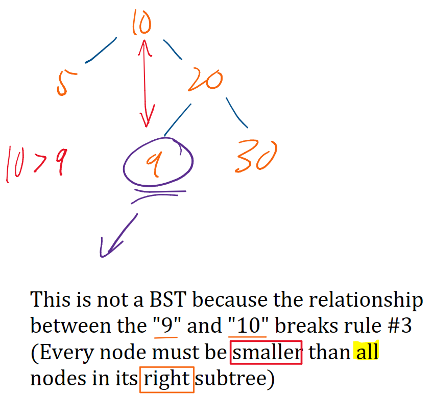
• Right Subtree Rule: All elements residing within its right subtree must hold values strictly larger than the node’s own key.

                  [ 50 ]
                 /      \
             [ 30 ]    [ 70 ]
            /    \      /    \
         [ 20 ] [40]  [60]  [80]

Duplicate Constraints

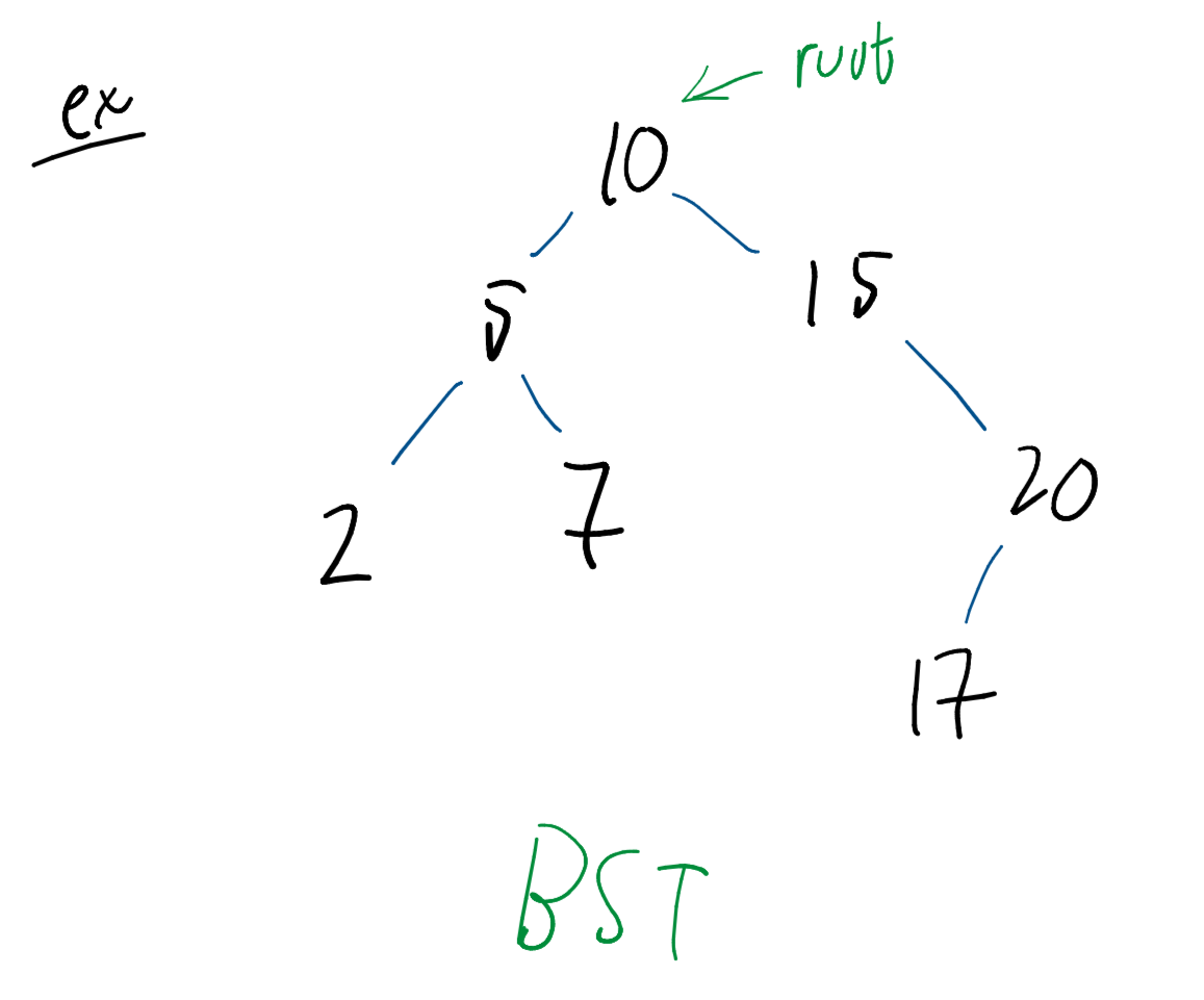
The strict inequality definitions of the BST property imply that the tree architecture cannot natively capture duplicate elements within its node paths.

Balanced Symmetrical Layout	Skewed Degenerate Layout

---

Data Structure Operations

The execution runtime of standard BST routines scales proportionally with the maximum height ($h$) of the tree block.

Find(element)

Traces downward from the root, branching left if the target value is smaller than the current node key or right if it is larger.

• Time Complexity: $O(h)$ operations.

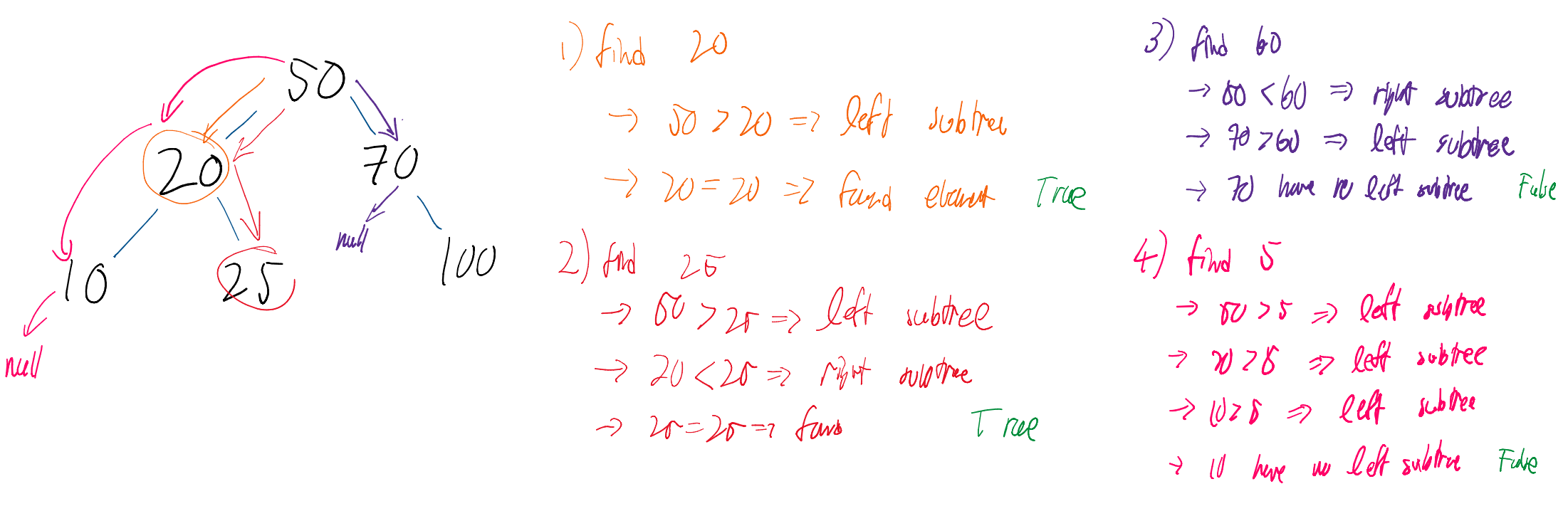
Algorithm 31 BST Value Search

procedure Find($element, root$)

$current \gets root$

while $current \neq \text{NULL}$and$current.\text{data} \neq element$ do

if $element < current.\text{data}$ then

$current \gets current.\text{leftChild}$

else

$current \gets current.\text{rightChild}$

return $current \neq \text{NULL}$

Insert(element)

Traverses down branching pathways to discover an available NULL child reference slot where the incoming element logically fits, appending it as a new leaf node.

• Time Complexity: $O(h)$ operations.

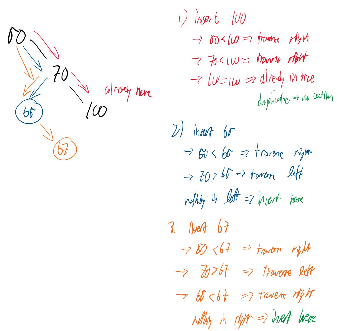
Algorithm 32 BST Leaf Insertion

procedure Insert($element, root, size$)

if $root == \text{NULL}$ then

$root \gets \text{CreateNode}(element)$

$size \gets size + 1$

return $\text{true}$

$current \gets root$

while $current.\text{data} \neq element$ do

if $element < current.\text{data}$ then

if $current.\text{leftChild} == \text{NULL}$ then

$current.\text{leftChild} \gets \text{CreateNode}(element)$

$size \gets size + 1$

return $\text{true}$

else

$current \gets current.\text{leftChild}$

else

if $current.\text{rightChild} == \text{NULL}$ then

$current.\text{rightChild} \gets \text{CreateNode}(element)$

$size \gets size + 1$

return $\text{true}$

else

$current \gets current.\text{rightChild}$

return $\text{false}$

Administrative Interface Metrics

• clear(): Resets the collection by severing the root pointer reference and resetting tracking allocations:
  $\text{root}=\text{NULL},\text{size}=0$
• size(): Returns the total active node count.
• empty(): Evaluates true if size == 0.

---

Successor and Removal Structural Logic

Finding the In-Order Successor

The in-order successor of a node $u$ represents the node holding the next largest key value across the entire tree sequence.

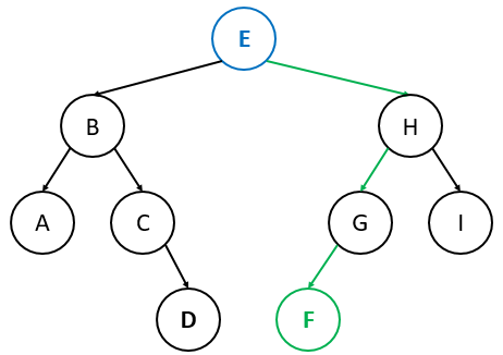
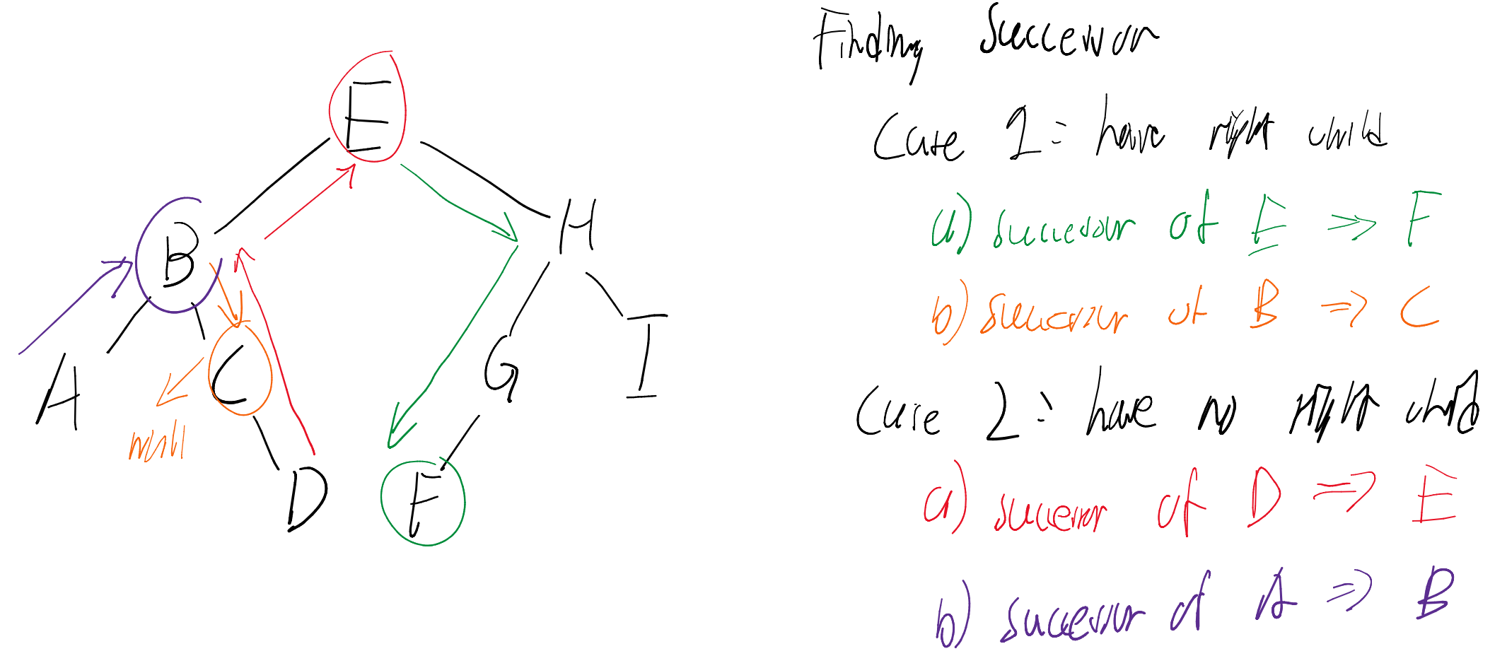
• Case 1 (Right Subtree Exists): The successor is located at the absolute left-most node coordinate of $u$‘s right subtree branch.
  
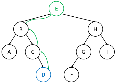
• Case 2 (No Right Subtree): Trace upward toward the root until encountering an ancestor node that acts as the left child of its parent. That specific parent node is the successor.
  

Algorithm 33 In-Order Successor Resolution

procedure Successor($u$)

if $u.\text{rightChild} \neq \text{NULL}$ then

$current \gets u.\text{rightChild}$

while $current.\text{leftChild} \neq \text{NULL}$ do

$current \gets current.\text{leftChild}$

return $current$

else

$current \gets u$

while $current.\text{parent} \neq \text{NULL}$ do

if $current == current.\text{parent}.\text{leftChild}$ then

return $current.\text{parent}$

$current \gets current.\text{parent}$

return $\text{NULL}$

Removal Cases

Erasing a node requires structural reorganization depending on child density:

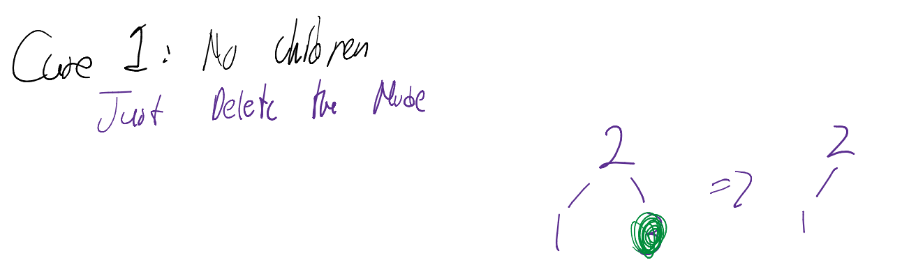
1. Zero Children (Leaf Node Removal): Simply delete the node and set the parent’s matching child pointer reference to NULL.
   
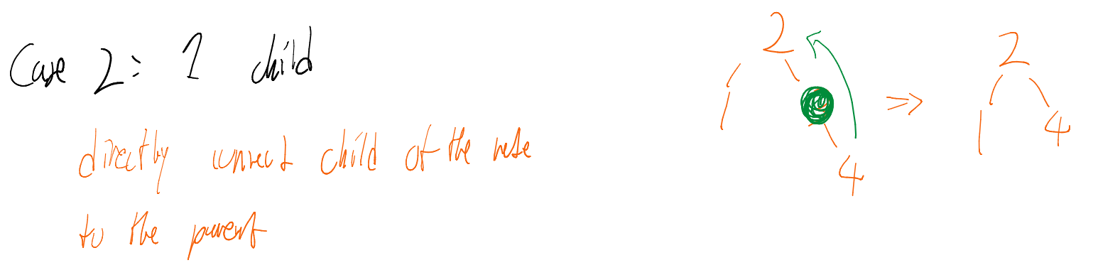
2. One Child Leaf Node Promotion: Splice the isolated node out by mapping its parent’s child reference directly to the node’s single child.
   
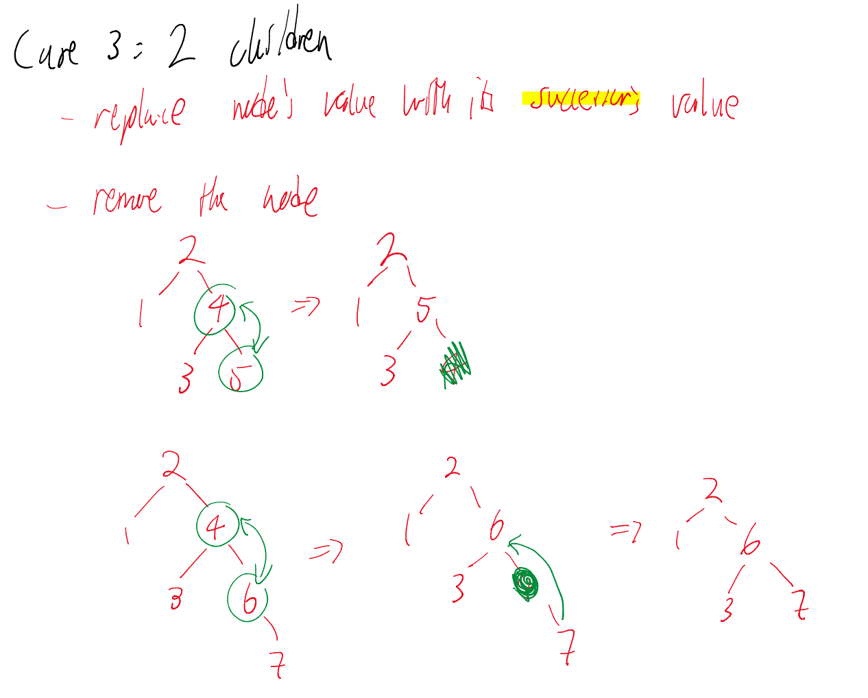
3. Two Children Substitution: Locate the node’s in-order successor. Overwrite the target node’s value with the successor’s key, then execute a sub-removal routine to drop the successor node (which is mathematically guaranteed to possess at most one child).
   

Algorithm 34 BST Node Removal

procedure Remove($element, root$)

$current \gets \text{LocateNode}(element, root)$

if $current == \text{NULL}$ then

return $\text{false}$

if $current.\text{leftChild} == \text{NULL}$and$current.\text{rightChild} == \text{NULL}$ then

DisconnectFromParent(current)

else if $current.\text{leftChild} == \text{NULL}$or$current.\text{rightChild} == \text{NULL}$ then

BypassNodeWithChild(current)

else

$s \gets$ Successor(current)

$savedVal \gets s.\text{data}$

Remove($s.\text{data}, root$)

$current.\text{data} \gets savedVal$

return $\text{true}$

---

Sequence Traversals

An In-Order Traversal walks the tree layout following the structural sequence: Left Subtree $\to$ Current Node $\to$ Right Subtree. This specific traversal is guaranteed to encounter items in perfectly sorted ascending sequence.

Algorithm 35 In-Order Successor Traversal Walk

procedure InOrderTraversal($root$)

$current \gets root$

while $current.\text{leftChild} \neq \text{NULL}$ do

$current \gets current.\text{leftChild}$

while $current \neq \text{NULL}$ do

Output($current.\text{data}$)

$current \gets$ Successor($current$)

---

Sizing Performance and Tree Shapes

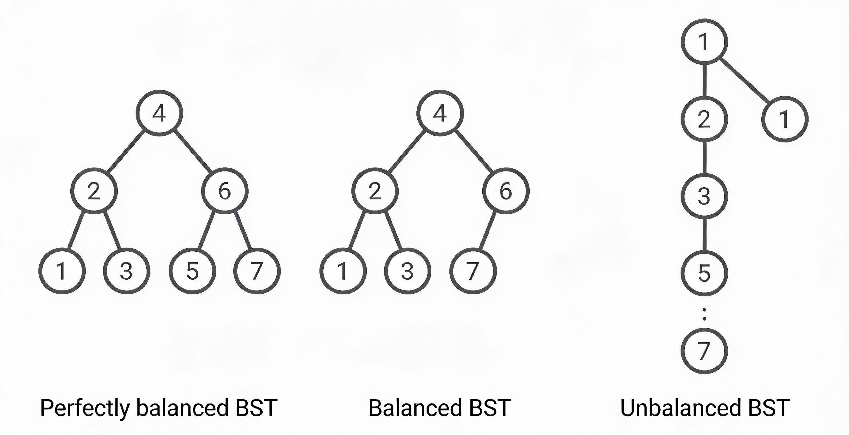
The operational utility of a standard BST relies entirely on its physical geometric shape, which is dictated by the chronological sequence of item insertions.

• Tree Height Configuration ($h$): Measured as the count of structural edge jumps separating the root from the deepest leaf node. An empty tree sets $h=-1$; a single isolated node sits at $h=0$; a worst-case unbalance peaks at $h=n-1$.

The Core Tree Balance Configurations

Feature Parameter	Perfectly Balanced Shape	Self-Balancing (AVL / Red-Black)	Degenerate (Skewed Chain)
Structural Layout	Full symmetrical triangle topology	Mostly full; bounded height variances	A straight linear line arrangement
Operational Logic	Levels fill completely before jumping down	Height constraints are dynamically managed	Elements land on one side exclusively
Height Bound	$h\approx {\log }_{2}n$	$h=O(\log n)$	$h=n-1$
Search Time	$O(\log n)$	$O(\log n)$ guaranteed worst-case	$O(n)$ linear scan bottleneck
Production Context	Complex/Costly to enforce perfectly	Industry standard default models	Triggered by sorting data streams

The Sorted Insertion Trap

Introducing sorted array streams (such as [1, 2, 3, 4, 5]) directly into a naive BST causes the structure to grow exclusively in one direction. This turns your search tree into an expensive, linear linked list layout. Production systems avoid this issue by implementing self-balancing tree architectures like AVL Trees to force geometric balance via structural rotations.

---

Average-Case Performance Analysis

While a naive insertion path can degrade to a worst-case $O(n)$ footprint, its average-case behavior across random distributions matches a highly efficient $O(\log n)$ curve.

1. Underlying Statistical Assumptions

To prove average-case performance bounds, we establish two constraints:

1. Uniform Search Distribution: Every element tracking inside the tree has an equal likelihood of being selected during a lookup query.
2. Uniform Insertion Sequence: All $n!$ possible insertion permutations of the target set have an equal probability of occurring.

2. Defining Expected Node Depth

We define the depth of node $i$ ($d_i$) as the count of node blocks on the path tracking from the root to node $i$. The root sits at depth 1. The expected total depth across a given tree structure $j$ resolves to:

$E_j(d)=\frac{1}{n}{\sum }_{i=1}^n{d}_{ji}=\frac{1}{n}{D}_j(n)$

where $D_j(n)$ represents the combined aggregate depth of tree configuration $j$.

3. The Structural Recurrence Model

Instead of evaluating all $n!$ layout shapes individually, we construct a structural recurrence relation modeled on the root element placement. If the root occupies the $(i+1)$-th smallest sorted coordinate position, then exactly $i$ nodes settle inside the left subtree branch, leaving $(n-i-1)$ nodes in the right subtree branch.

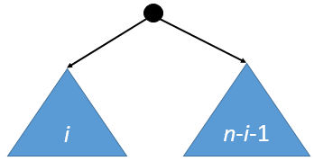
The expected aggregate depth calculation given a subtree density split of $i$ items maps to:

$D(n\mid i)=D(i)+D(n-i-1)+n$

(The $+n$ factor accounts for the structural constraint that appending a root node shifts every nested subtree node exactly one level deeper).

Since each element has an equal probability of being selected as the first item inserted (assuming the root position), the probability of choosing any subtree configuration $i$ tracks to $\frac{1}{n}$. This gives us the following recurrence relation:

$D(n)=\frac{2}{n}{\sum }_{i=0}^{n-1}D(i)+n$

4. Mathematical Solution Proof

Multiplying the recurrence layout expression by $n$ yields:

$nD(n)=2{\sum }_{i=0}^{n-1}D(i)+n^2\text{— (Equation 1)}$

Substituting the parameter size boundary to $(n-1)$ produces:

$(n-1)D(n-1)=2{\sum }_{i=0}^{n-2}D(i)+(n-1{)}^2\text{— (Equation 2)}$

Subtracting Equation 2 from Equation 1 simplifies the summation chain down to a telescoping form:

$nD(n)-(n-1)D(n-1)=2D(n-1)+n^2-(n-1{)}^2$

$nD(n)=(n+1)D(n-1)+2n-1$

Solving this relation yields the exact closed-form depth solution for the structure:

$D(n)=2(n+1){\sum }_{i=1}^n\frac{1}{i}-3n$

5. Final Harmonic Approximation

Applying the standard harmonic series expansion approximation (${\sum }_{i=1}^n\frac{1}{i}\approx \ln n$), the expected average count of character comparisons for a lookup query matches:

$\frac{D(n)}{n}\approx 2\ln n\approx 1.386{\log }_{2}n$

Because the multiplier $1.386$ is a fixed constant coefficient, this proves that the average-case runtime complexity for a standard binary search tree is strictly bounded at $O(\log n)$.

---

Related Notes

• AVL Tree
• Binary Search Tree Implementation
• Priority Queue
• Binary Tree