Strongly Connected Components

Abstract

Two vertices $u$ and $v$ in a directed graph are strongly connected if there exists a path from $u$ to $v$ and a path from $v$ to $u$. The maximal set of strongly connected vertices is called a Strongly Connected Component (SCC). Every directed graph is a DAG of its SCCs, so some SCCs are sink SCCs and some are source SCCs.

• Category: Graph Algorithm (directed graphs)
• Input: Directed graph $G=(V,E)$
• Output: A partition of $V$ into its strongly connected components
• Paradigm: Two-pass DFS, using a reversed graph
• Typical use cases: condensing a directed graph into its DAG-of-SCCs structure, dependency/cycle analysis

---

Core Logic (High-Level)

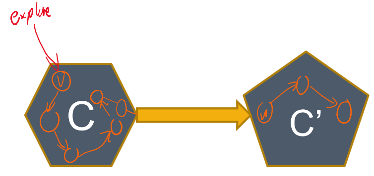
There is a linear-time algorithm that decomposes a directed graph into its SCCs. If Explore is performed on a vertex $u$, it visits only the vertices reachable from $u$. If $u$ is in a sink SCC, running explore on $u$ reaches exactly the nodes in that SCC — nothing more, since a sink SCC has no outgoing edges to other SCCs.

This suggests a way to look for SCCs:

1. Start explore on a vertex in a sink SCC and visit its SCC.
2. Remove the sink SCC from the graph and repeat.

Key Idea

The problem is finding a vertex in a sink SCC in the first place — there’s no direct way to spot one. But there is a direct way to find a vertex in a source SCC (see Proof below), and a sink of $G$ is just a source of the reversed graph $G^R$. So: run DFS on $G^R$ to find sink SCCs of $G$, then use that order to peel off SCCs of $G$ one at a time.

---

Pseudocode (Mid-Level Implementation)

Algorithm 40 SCC

Input: Directed graph $G = (V,E)$

Output: Partition of $V$ into strongly connected components

procedure SCC($G$)

Construct $G^R$, the reverse of $G$

Run DFS on $G^R$, recording $post(v)$ for every vertex

Run DFS on $G$, considering vertices in decreasing order of $post(v)$ from the previous step

Note

Every time DFS increments $cc$, a new SCC has been found

Variables & Data Structures

Name	Type	Purpose
G^R	Graph (reversed adjacency)	Same vertices as $G$, every edge direction flipped; sources of $G^R$ = sinks of $G$
post(v)	Array (vertex → int)	Finish timestamp from the first DFS, run on $G^R$; determines processing order for the second DFS
cc	Integer counter	Incremented once per explore call in the second DFS — each increment marks the discovery of one new SCC

Helper Functions / Operations Used

• DFS / explore — see Depth First Search (DFS) and Explore for the underlying traversal and post timestamp mechanics used here
• Reverse graph construction — build $G^R$ by flipping every edge $(u,v)\to (v,u)$; $O(|V|+|E|)$

---

Proof of Correctness

Property (Generalized)

Claim: If $C$ and $C^{\prime }$ are strongly connected components and there is an edge from a vertex in $C$ to a vertex in $C^{\prime }$, then the highest post number in $C$ is greater than the highest post number in $C^{\prime }$.

Case 1: DFS searches $C$ before $C^{\prime }$. At some point DFS will cross into $C^{\prime }$ and visit every vertex in $C^{\prime }$, then retrace its steps back to the first node in $C$ it started with, assigning that node the highest post number in $C$ only after all of $C^{\prime }$ has already been finished.

• $v$: the last vertex removed from visited (highest post number)
• $u$: a vertex popped before $v$ does

Case 2: DFS searches $C^{\prime }$ before $C$. DFS will visit all vertices of $C^{\prime }$ before getting stuck (since a sink-ward SCC like $C^{\prime }$ here can’t lead back into $C$) and assign post numbers to all of $C^{\prime }$. Only later does it visit some vertex of $C$ and assign post numbers to those vertices — so $u$ (in $C^{\prime }$) is popped first, and $v$ (in $C$) is pushed and popped later, giving $post(v)>post(u)$.

Either way, the highest post number belongs to a vertex in $C$, confirming the claim.

Conclusion: Linearization

The SCCs can be linearized by arranging them in decreasing order of their highest post numbers. In particular:

The vertex with the greatest post number in any [DFS Output Tree](Explore#DFS Output Tree) belongs to a source SCC.

This follows directly from the Property above: a source SCC has no incoming edges from any other SCC, so no other component’s highest post number can exceed its own.

Finding Sink SCCs via the Reverse Graph

Given $G$, let $G^R$ be its reverse. Then the sources of $G^R$ are the sinks of $G$. So:

• Running DFS on $G^R$ and taking the vertex with the highest post number gives a vertex in a source of $G^R$ — which is a sink of $G$.
• Start explore on this vertex (in $G$) to find that whole SCC.
• The vertex with the next-greatest post number in $G^R$ (among vertices not yet visited) is in the next SCC in linear order — repeat from there.

This is exactly the peeling process from Core Logic, made concrete: the second DFS (on $G$, run in decreasing order of $G^R$‘s post numbers) never “leaks” from one SCC into an unprocessed one, because by the time it reaches a given vertex, every SCC that could pull it further has already been fully explored and marked visited in an earlier explore call.

---

Time & Space Complexity Analysis

General Case

	Complexity	Notes
Time	$O(\Vert V\Vert +\Vert E\Vert )$	Three linear-time passes, summed:

1. Construct $G^R$ → $O(|V|+|E|)$
2. DFS on $G^R$ → $O(|V|+|E|)$
3. DFS on $G$ → $O(|V|+|E|)$

Therefore the total time complexity of the SCC algorithm is linear: $O(|V|+|E|)$.

	Complexity	Notes
Space	$O(V+E)$	Adjacency lists for both $G$ and $G^R$, plus the post array and visited/cc bookkeeping from the two DFS passes

Best / Worst / Average Case

• Best / Worst / Average case: All $O(|V|+|E|)$ — every step is a full graph traversal or construction; there’s no early exit, since the algorithm must find every SCC, not just one.

---

Drawbacks / Constraints

• Only meaningful for directed graphs. Strong connectivity collapses to ordinary connectivity on an undirected graph, so this algorithm’s structure (source/sink SCCs, reverse graph) is specific to directed inputs.
• The naive approach doesn’t work: the vertex with the least post number in a single DFS output tree on $G$ does not necessarily belong to a sink SCC — this is why the reverse-graph trick (finding sources of $G^R$, i.e. sinks of $G$) is needed instead of trying to read sinks directly off one DFS pass on $G$.
• Requires building $G^R$ explicitly (or an equivalent reverse-adjacency structure), adding $O(V+E)$ extra space beyond just $G$ itself.

---

References / Links

• Explore
• Depth First Search (DFS)
• Graph Reachability