Binary Search

Abstract

Binary Search is only applicable if the list is sorted. It uses the “Decrease and Conquer” strategy to eliminate half of the search space with every comparison.

• Category: Searching / Decrease and Conquer
• Input: Target value $x$; a sorted (increasing order) array $[a_1,a_2,\dots ,a_n]$
• Output: The index of $x$ in the array, or an indication that it’s not present
• Paradigm: Decrease and Conquer (each step shrinks the problem by a constant fraction, rather than splitting into multiple independent subproblems like Divide and Conquer does)
• Typical use cases: searching sorted arrays, finding insertion points, as a building block for range queries and lower/upper-bound lookups

---

Core Logic (High-Level)

1. Divide: Identify the mid-point of the current list. Divide the search space into two conceptual halves:
   • $[0,\text{mid-point})$ — the left half.
   • $[\text{mid-point}+1,n)$ — the right half.
2. Compare: Check the target element against the value at the mid-point:
   • Smaller: search the left half.
   • Greater: search the right half.
   • Equal: return the current position (target found).
3. Recurse: continue splitting and searching until only one element remains.
4. Terminate: if the search space is exhausted without a match, report that the item is not found.

Key Idea

Because the list is sorted, comparing against a single mid-point tells you which entire half can be safely thrown away — you never need to check it. That’s what makes this “decrease” rather than “divide”: only one half is ever explored, not both.

---

Pseudocode (Mid-Level Implementation)

Algorithm 6 Binary Search

Input: $x$: integer to search for

Input: $[a_1, a_2, \dots, a_n]$: array of increasing ordered integers to search in

Output: Index of where the interger is in the array ($0$ if input not in array)

procedure BinarySearch($x, [a_1, a_2, \dots, a_n]$)

$lo = 1$

$hi = n$

while $lo \leq hi$ do

$m = \lceil \frac{(lo + hi)}{2} \rceil$

if $x == a_m$ then

return $m$

if $x < a_m$ then

$hi = m-1$

if $x > a_m$ then

$lo = m+1$

return $0$

Variables & Data Structures

Name	Type	Purpose
lo, hi	Integer indices	Bound the current search space $[lo,hi]$ (inclusive, 1-indexed here); the loop narrows this range every iteration
m	Integer index	The current mid-point being compared against; $\lceil (lo+hi)/2\rceil$
x	Value	The target being searched for
a	Sorted array	The list being searched; requires $O(1)$ random access by index

Index Convention

This pseudocode is 1-indexed ($lo$ starts at 1), while the conceptual “Divide” step above describes the halves as $[0,\text{mid-point})$ and $[\text{mid-point}+1,n)$ using 0-indexing. Both describe the same idea — just double check which convention you’re using when implementing, since off-by-one errors here are the single most common bug in binary search.

Helper Functions / Operations Used

• Random access a[i] — must be $O(1)$; this is the one hard requirement on the data structure (see Drawbacks / Constraints).
• Ceiling division ⌈(lo+hi)/2⌉ — picks the upper mid-point on ties; picking the floor instead also works, as long as the corresponding bound updates (hi = m-1 / lo = m+1) stay consistent with whichever rounding you chose, to guarantee the range always shrinks.

Low-Level Implementation

The version above is iterative, using $O(1)$ extra space. A recursive version is often written to mirror the inductive proof below directly (call on the sub-array of size $\approx n/2$), but that costs $O(\log n)$ extra space for the recursion stack — see Time & Space Complexity Analysis.

---

Proof of Correctness

Claim: Binary Search correctly finds the target in a sorted list of size $n$ (proof by strong induction on $n$).

• Base Case ($n=1$): the mid-point is the only element. The algorithm checks it directly and correctly returns the index or reports “not found.”
• Inductive Hypothesis: assume Binary Search is correct for all sorted lists of size $m<n$.
• Inductive Step: for a list of size $n$, the algorithm compares against the mid-point.
  • If equal, it returns correctly.
  • If not equal, it recurses on a sub-list of size roughly $n/2$ — and since the list is sorted, the target (if present) is guaranteed to be entirely within whichever half was kept, never the discarded half.
  • Since $n/2<n$, the Inductive Hypothesis applies, and the sub-search is guaranteed to be correct.

Termination: each iteration strictly shrinks the range — $hi-lo$ decreases every time, since either hi = m-1 < m ≤ hi or lo = m+1 > m ≥ lo. So after finitely many iterations, either the target is found, or $lo>hi$ and the loop exits, correctly reporting “not found” since every remaining candidate has been ruled out by the sorted-order comparisons along the way.

---

Time & Space Complexity Analysis

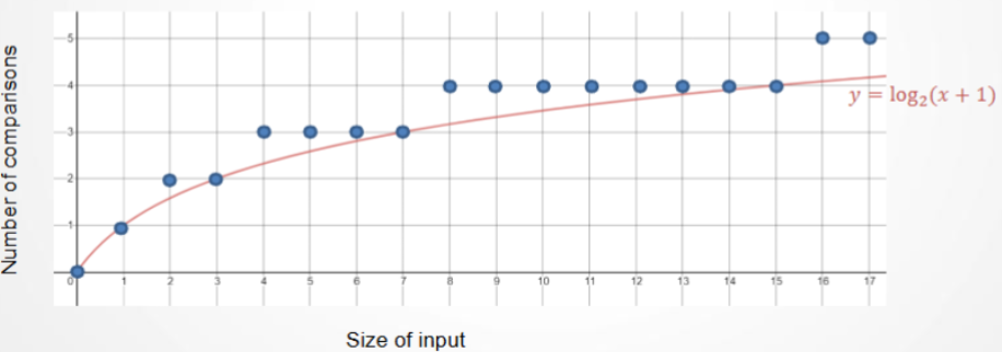
The efficiency of Binary Search comes from how quickly it shrinks the input. Each “split” reduces the remaining work by half.

Comparison Scaling

As the input size $n$ roughly doubles, the number of required comparisons only increases by 1:

n	# of splits	# of comparisons (k)
1	0	1
3	1	2
7	2	3
15	3	4
31	4	5

Deriving the Complexity

If the list size is $n=2^k-1$, you need $k$ comparisons. Solving for $k$ in terms of $n$:

\begin{align*} n &\leq 2^k - 1 \ n+1 &\leq 2^k \ \log_{2}(n+1) &\leq k \ k &= \boxed{\lceil\log_{2}(n+1)\rceil} \end{align*}

This confirms that Binary Search grows at a logarithmic rate, $O(\log n)$, making it incredibly efficient for large datasets.

General Case

	Complexity	Notes
Time	$O(\log n)$	Each comparison eliminates half the remaining search space
Space	$O(1)$ iterative / $O(\log n)$ recursive	Iterative version only needs lo, hi, m; recursive version accumulates one stack frame per halving

Implementation-Dependent Variations

Data Structure Choice	Impact on Time	Impact on Space	Notes
Array (contiguous, random access)	$O(\log n)$ total	$O(1)$	The standard case — this is what makes $O(1)$ mid-point access possible
Linked List	$O(n\log n)$ total — finding each mid-point takes $O(n)$ since there’s no random access	$O(1)$	Effectively defeats the purpose of binary search; see Drawbacks
Iterative vs. recursive	Same asymptotic time	$O(1)$ vs. $O(\log n)$	Recursive is closer to the inductive proof’s structure but costs stack space

Best / Worst / Average Case

• Best case: $O(1)$ — the target happens to be exactly at the first mid-point checked.
• Worst case: $O(\log n)$ — target is not present, or is found only at the very last possible comparison.
• Average case: $O(\log n)$ — dominated by the same halving regardless of where the target sits, since even a “lucky” run only saves a constant number of comparisons off the $\log n$ bound.

---

Drawbacks / Constraints

• Preconditions: the list must already be sorted. If it isn’t, Binary Search’s comparisons give no reliable information about which half to discard, and it will silently produce wrong results rather than erroring out.
• Requires $O(1)$ random access. Data structures without indexed access (e.g. a linked list) force $O(n)$ just to locate each mid-point, which erases the entire benefit — use a structure like an array, or a balanced BST if the data also needs to change frequently.
• Not suitable for: frequently-changing (dynamic) datasets, since keeping an array sorted after insertions/deletions costs $O(n)$ per update to shift elements. A balanced BST (or skip list) supports both $O(\log n)$ search and $O(\log n)$ insert/delete, at the cost of not being a flat array.
• Alternatives to consider: a hash table for $O(1)$ average lookup when you don’t need sorted order or range queries at all; Computer Science Theory/Discrete Structures/Discrete Algorithms/Recursive Algorithms/Divide and Conquer/Merge Sort (or any $O(n\log n)$ sort) as the standard way to get a list sorted in the first place before searching it.

---

References / Links

• Linear Search vs Binary Search — visualizing why $O(\log n)$ is asymptotically faster.
• Computer Science Theory/Discrete Structures/Discrete Algorithms/Recursive Algorithms/Divide and Conquer/Merge Sort — the most common way to ensure a list is sorted before searching.
• Asymptotic Notation — more on the $O$ notation used here.