Graph Algorithm Approaches

Overview

When you have a new problem to solve and you already have an algorithm that solves a related problem, there are two general strategies for building an algorithm out of it:

1. Modification — change the existing algorithm’s internal logic so it directly tracks/solves the new problem.
2. Reduction — leave the existing algorithm untouched, and instead transform the input of the new problem into an instance of the old one, calling the existing algorithm as a subroutine.

This note works through both strategies using the Max Bandwidth Problem as a running example.

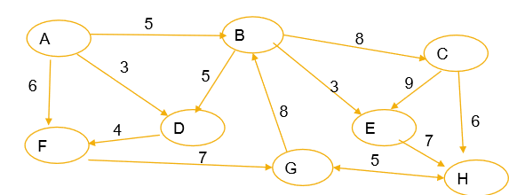
Driving Example: Max Bandwidth Problem Graph represents a network, with edges representing communication links. Edge weights are the bandwidth of the link — what is the largest bandwidth of a path from $A$ to $H$?

---

Defining the Problem Formally

Before picking a strategy, it helps to pin down the problem precisely. Any optimization problem can be broken into 4 parts:

1. Instance (Input): what you’re given.
2. Solution Type (Output): the shape of the answer.
3. Constraints: what must be true of a valid answer.
4. Objective: what you’re optimizing over all valid answers.

Driving Example — Max Bandwidth, formalized:

1. Instance: Directed graph $G=(V,E)$ with positive edge weights $w(e)$, two vertices $s,t\in V$.
2. Solution Type: A sequence of edges.
3. Constraints: The sequence of edges is a path $p$ from $s$ to $t$ in $G$.
4. Objective: Over all possible paths $p$ between $s$ and $t$, find one that maximizes the bandwidth of a path:

$BW(p)=\underset{e\in p}{\min }w(e)$

---

Approach 1: Algorithm Modification

Take an existing algorithm that solves a structurally similar problem, and change what it tracks internally so it solves the new problem instead — e.g. starting from Graph Search and having it track a new quantity per vertex instead of just visited/unvisited.

Limitations

1. Runtime is no longer guaranteed to match the original — it must be reanalyzed from scratch.
2. The modified algorithm is not automatically correct just because the original was — it must be reproven, in full, from the ground up.

Driving Example: Max Bandwidth via Modification

Use the basic structure of Graph Search, and for each vertex $v$, keep track of the max bandwidth to $v$ found so far. Then move a vertex into $F$ only if its max bandwidth has improved.

Algorithm 36 Max Bandwidth Modify Algorithm Approach

procedure MaxBand1($G: \text{directed graph}, s, t$)

Initialize $X$ = emtpy, $F = \{s\}$

B($v$) = 0 for $v \in V$

B($s$) = $\infty$

while $F$ is not empty do

Pick $v$ in $F$

for each neighbor $u$ of $v$ do

$m$ = min(B($v$), w($v, u$))

if $m >$ B($u$) then

move $u$ to $F$

B($u$) = $m$

move $v$ from $F$ to $X$

return B($t$)

Variables: $B(v)$ — the bandwidth of the best path found so far from $s$ to $v$.

Proof of Correctness

Note this whole proof is only necessary because this is a modification — nothing about Graph Search’s original correctness proof transfers over automatically.

Claim: At the end of the algorithm, $B(v)$ is the maximum bandwidth from $s$ to $v$, for all vertices $v\in V$.

Part 1 — $B(v)$ is always achievable: for all $v\in V$, there is a path $p$ from $s$ to $v$ such that $BW(p)=B(v)$.

• Loop Invariant: after every iteration, for all $v$, there is a path from $s$ to $v$ with $BW(p)=B(v)$.
• Base Case: before the first iteration, $B(s)=\infty$ and $B(v)=0$ for every other vertex.
• Inductive Hypothesis: assume the claim holds after $t$ iterations.
• Inductive Step: pick $v$ in $F$, let $u$ be a neighbor of $v$, and $m=\min (B(v),w(v,u))$.
  • Case 1: $m\le B(u)$ — $B(u)$ doesn’t change.
  • Case 2: $B(u)<m$ — $B(u)$ updates to $m$.
  • Either way, there still exists a path from $s$ to $u$ with bandwidth exactly $B(u)$.
• So the loop invariant holds after every iteration, including the last — meaning by the end, every vertex $v$ has a real path from $s$ to $v$ achieving bandwidth $B(v)$.

Part 2 — $B(v)$ is never an underestimate: for all $v\in V$, $B(v)$ is the maximum bandwidth among all paths from $s$ to $v$ (not just some achievable value).

• Suppose by contradiction there’s a vertex $v$ with some path $p$ from $s$ to $v$ where $BW(p)>B(v)$. Let $b=BW(p)$.
• Let $y$ be the first vertex along $p$ where $B(y)<b$, and $z$ the vertex right before $y$ on $p$ (so $B(z)\ge b$).
• Since $p$ has bandwidth $b$, every edge on it — including $(z,y)$ — has weight $\ge b$, so $w(z,y)\ge b$.
• When $z$ is processed, the algorithm computes $m=\min (B(z),w(z,y))\ge b$. Since $B(y)<b\le m$, the algorithm updates $B(y)$ to $m\ge b$.
• This contradicts the assumption that $B(y)<b$ at the end of the algorithm. $■$

---

Approach 2: Reduction

What is a Reduction?

Instead of modifying an existing algorithm, we modify the input so we can use the existing algorithm as a subroutine. We map instances of one problem to instances of another, then use any known algorithm for that second problem as a subroutine to build an algorithm for the first — the existing algorithm’s correctness and runtime proofs carry over unchanged.

Reduction From a Decision Version

A useful general pattern: to relate a decision problem to an optimization problem, look at the decision version of the optimization problem instead of the optimization problem itself. A decision version asks a yes/no question (“is there a solution at least this good?”) rather than “find the best solution” — and it’s often much easier to reduce to something else.

Driving Example: Max Bandwidth via Reduction

Decision Version of Max Bandwidth: Given $G,s,t,M$, is there a path of bandwidth $M$ or better from $s$ to $t$?

Algorithm 37 Max Bandwidth Reduction Approach

procedure MaxBandDecision($G, s, t, M$)

Construct $G_M$ by removing all edges less than $M$ from $G$

Run graphSearch($G_M, s$)

if $t$ is visited then

return true

else

return false

The transformation itself — building $G_M$ — is the entire reduction. Graph Search runs completely unmodified on $G_M$.

Proof of Correctness

Note how much smaller this proof is compared to the Modification approach — we only need to prove the reduction step correct, since graphSearch itself is already proven correct elsewhere.

Direction 1 — if there’s a path in $G$ with bandwidth $\ge M$, the algorithm returns TRUE: Suppose path $p$ in $G$ from $s$ to $t$ has bandwidth at least $M$. Then every edge in $p$ has weight $\ge M$, so $p$ survives entirely in $G_M$ (no edge of $p$ gets removed). So graphSearch visits $t$, and the algorithm outputs TRUE.

Direction 2 — if there’s no such path, the algorithm returns FALSE: Restated as the contrapositive: if the algorithm returns TRUE, then there is a path from $s$ to $t$ in $G$ with bandwidth at least $M$. Suppose the algorithm returns TRUE. Then there’s a path $p$ in $G_M$ from $s$ to $t$. Every edge in $G_M$ has weight $\ge M$ by construction, so $p$ is also a path in $G$ where every edge weight is $\ge M$ — meaning $BW(p)\ge M$ in $G$ as well.

Time Analysis

Let $n=|V|,m=|E|$.

• Time to construct $G_M$: $O(n+m)$
• Time to run graphSearch (already analyzed, unchanged): $O(n+m)$

Total Time: $O(n+m)$ — note this reuses graphSearch’s existing runtime bound rather than re-deriving it.

To solve the full optimization problem (not just the decision version), binary search over candidate values of $M$ (e.g. the distinct edge weights) and call MaxBandDecision at each — this reuses the decision procedure as a subroutine without needing a new correctness proof for the search itself.

---

Comparing the Two Approaches

	Modification	Reduction
What changes	The existing algorithm’s internal logic	The input, via a transformation step; the existing algorithm runs unchanged
Correctness burden	Reprove the entire modified algorithm from scratch	Only prove the transformation step correct — the existing algorithm’s proof carries over
Runtime burden	Reanalyze the runtime of the modified algorithm	Runtime = cost of the transformation + the existing algorithm’s already-known runtime
Reusability	A one-off algorithm specific to this problem	Any correct, analyzed algorithm for the target problem can be swapped in
Max Bandwidth outcome	New proof (2 parts, induction) + new complexity argument	Reduction proof (2 directions) + graphSearch’s complexity reused as-is

---

When to Use Which

• Prefer Reduction when a well-analyzed algorithm already exists for a problem your new problem’s decision version (or some other variant) can be mapped onto — you inherit its correctness and runtime for free, paying only for the transformation.
• Reach for Modification when no existing algorithm is close enough to reduce to, or when the transformation needed for a reduction would itself be as expensive or as hard to prove correct as just modifying the algorithm directly.
• Either way, the goal is the same: get to a fully specified, analyzed algorithm while doing as little new correctness/runtime work as possible.

---

References / Links

• Graph Reachability
• Levels of Algorithm Design