Graph Representations

Abstract

Mapping a structural network layout down into raw physical system memory requires balancing spatial footprint parameters with execution algorithm lookups. Realizing an implementation requires assessing edge density trends to properly select between an Adjacency Matrix and an Adjacency List.

Category: Graph Representation Formats
Stores: Directed or undirected node-to-edge connectivity mappings.
Typical use cases: Route optimization inside geographic mapping software, graph analysis, circuit board link arrays.

---

Core Structure: Density vs. Sparsity

Selecting the ideal representation layout requires comparing the active edge count $|E|$ against the maximum possible mathematical allocation threshold of a given node array.

• Maximum Boundary Limit: In a graph structure bounding $|V|$ total vertices, if every node retains a link to every other entry (including itself), total edge scale hits: $|E|{}_{max}=|V|{}^2$.
• Dense Graphs: Active link allocations approach the maximum limit ($|E|\approx |V|{}^2$). Under these parameters, matrix models perform exceptionally well.
• Sparse Graphs: The actual link footprint is significantly smaller than the quadratic limit ($|E|\ll |V|{}^2$). Real-world applications (e.g., road maps or social connection groups) are almost entirely sparse, making list models the standard choice.

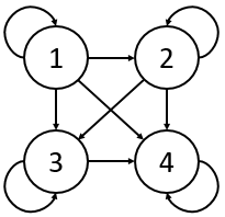
Dense Structural Topology.

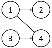
Sparse Structural Topology.

---

Data Structure Operations

The Adjacency Matrix

An Adjacency Matrix models a network layout utilizing a 2D square array allocation tracking dimensions of exactly $|V|\times |V|$.

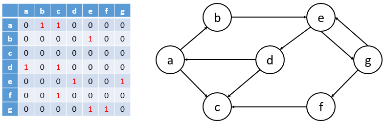
• Logic: Cell grid coordinates $M[i][j]$ commit a binary flag bit: 1 if a clean edge path extends from vertex $i$ to vertex $j$, and 0 otherwise.
• Weighted Variations: Replace the binary bit tokens with actual floating-point weight metrics (e.g., $M[i][j]=5.5$). Unconnected channels track infinity or sentinel markers.
• Space Bounds: Constant quadratic footprints: $O(|V|{}^2)$.

Key Idea

The adjacency matrix of an undirected graph is always symmetric across the diagonal ($M[i][j]==M[j][i]$) because an edge between $i$ and $j$ works in both directions.

The Adjacency List

An Adjacency List maps a graph configuration utilizing a 1D structural pointer array of size $|V|$, where each element links out to an independent variable-length collection or linear chain tracking its active neighbors.

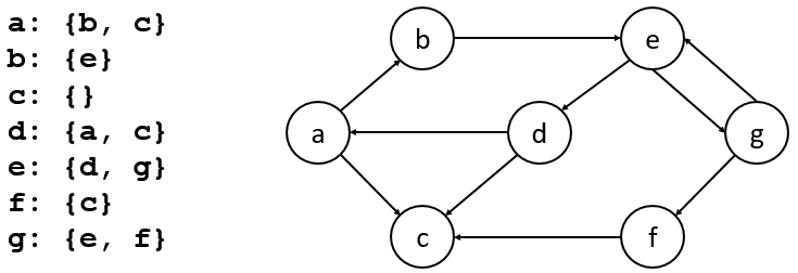
• Logic: If vertex 0 has path outputs extending to nodes 1 and 4, the list array head index 0 stores pointers leading to items [1, 4].
• Weighted Variations: Every link node inside a vertex chain stores a composite tuple tracking both the destination index and its associated edge weight.
• Space Bounds: $O(|V|+|E|)$.

---

Representation Comparison Matrix

Algorithmic Metric	Adjacency Matrix Strategy	Adjacency List Strategy
Ideal Deployment Target	Dense Graph Environments	Sparse Graph Environments
Memory Allocation Footprint	$O(|V|{}^2)$ — Heavy Fixed Overhead	$O(|V|+|E|)$ — Scaled to Size
Edge Verification: $\text{Query}(u,v)$	$O(1)$ — Absolute Constant Time	$O(\text{Degree}(u))$ — Bounds Linear Scan
Neighbor Discovery: $\text{GetNeighbors}(u)$	$O(|V|)$ — Must Scan Full Row	$O(\text{Degree}(u))$ — Reads Active Links Only
Vertex Insertion Overhead	$O(|V|{}^2)$ — Demands Full Matrix Realloc	$O(1)$ — Appends Head Pointer Array

---

Common Pitfalls

The Zero-Memory Waste Penalty

Deploying a 2D Adjacency Matrix to track a massive, sparse network will cause extreme memory waste. If a graph holds 100,000 nodes but every element links to only 3 neighbors, a matrix allocates 10 billion data blocks purely to store dummy zeros, crashing system memory footprints.

• Linear Scan Latency inside Lists: Looking up if a link exists between node $u$ and node $v$ drops from an instant $O(1)$ check down to a linear row scan bounded by the connectivity degree of node $u$.

---

Related Notes

• Graphs — The high-level theoretical framework mapping graph metrics.
• Minimum Spanning Trees — Demonstrates how representation performance metrics directly alter the runtimes of core network optimization passes.