Dijkstra's Algorithm

ABSTRACT

While BFS finds the shortest path in unweighted graphs (least number of edges), it fails when edges have varying costs. Dijkstra’s Algorithm is a Greedy Algorithm that solves the Single-Source Shortest Path problem for weighted graphs, provided all edge weights are non-negative.

• Category: Graph Traversal / Greedy Algorithm
• Input: Directed graph $G$ with edge weights $\ell$, source vertex $s$
• Output: dist(v) — the shortest total weight from $s$ to every vertex $v$
• Paradigm: Greedy, priority-queue-driven frontier expansion
• Typical use cases: shortest path in weighted graphs (non-negative weights), routing, network cost minimization

---

Core Logic: Greedy Shortest Path

Why BFS Fails on Weighted Graphs

BFS assumes that every edge has a cost of $1$. In a weighted graph, a path with more edges might actually have a lower total weight than a direct edge.

• BFS Path: $A\to C$ (Total Weight: 30)
• Shortest Weighted Path: $A\to B\to C$ (Total Weight: $12+5=17$)

Dijkstra’s Algorithm accounts for these costs by prioritizing paths with the smallest cumulative weight.

The Greedy Strategy

Dijkstra’s is a Greedy Algorithm. It makes the optimal choice at each step — picking the closest unvisited vertex — and assumes that this choice will lead to the overall shortest path.

Key Idea

1. Assign a Distance of infinity to all nodes, except the start node (which is 0).
2. Maintain a Priority Queue to store (distance, vertex) pairs.
3. Always “relax” the neighbor: if the path to a neighbor through the current node is shorter than its previously known distance, update its distance and add it to the PQ.
4. Once a node is “Done” (dequeued), its shortest path is guaranteed.

---

Pseudocode (Mid-Level Implementation)

High-Level Implementation

Dijkstra’s uses a Priority Queue to efficiently find the next vertex with the minimum distance.

Algorithm 29 Dijkstra's High Level

procedure Dijkstra's($G: \text{directed graph with edgeweights}, s: \text{vertex}$)

$X$ = empty, $F$ = $\{ s \}$

Initialize $dist(v) = \infty$ for all $v$

$dist(s) = 0$

while $F$ is not empty do

Pick $v$ in $F$ that has the $\underline{\text{lowest } dist(v) \text{ value}}$

for each neighbor $u$ of $v$ do

if $dist(u) > dist(v) + \ell(v, u)$ then

move $u$ to $F$

$dist(u) = dist(v) + \ell(v, u)$

move $v$ from $F$ to $X$

Variables & Data Structures

Name	Type	Purpose
X	Set	Vertices whose shortest distance is finalized (“Done”)
F	Set / Priority Queue	Frontier — vertices discovered but not yet finalized, keyed by dist
dist	Array (vertex → number)	Best known distance from $s$ to each vertex; starts at $\infty$ except $dist(s)=0$
prev	Array (vertex → vertex)	Predecessor pointer, used to reconstruct the shortest path (low-level version)
ℓ(v, u)	Edge weight function	The cost of traveling directly from $v$ to $u$

Helper Functions / Operations Used

• “Relax” an edge — if $dist(u)>dist(v)+\ell (v,u)$, update $dist(u)$ and re-prioritize it in the queue
• deletemin(H) — pop the vertex with the smallest current dist value
• decreasekey(H, v) — lower the priority (distance key) of v in the priority queue after a successful relaxation

Pick $v$ in $F$ carefully Dijkstra's Algorithm falls into a problem where vertices may re-enter $F$ more than once. If we pick $v$ in $F$ carefully (always the minimum dist), we can avoid this — this is exactly what a priority queue gives us for free.

Optional Low-Level Implementation Full implementation using an explicit priority queue with deletemin / decreasekey:

Algorithm 30 Dijkstra

procedure Dijkstra($G, \ell, s$)

for all $u \in V$ do

dist($u$) $:= \infty$

prev($u$) $:=$ null

dist($s$) $:= 0$

$H$ := makequeue($V$)

while $H$ is not empty do

$u :=$ deletemin($H$)

for all edges $(u, v) \in E$ do

if dist($v$) > dist($u$) + $\ell(u, v)$ then

dist($v$) $:=$ dist($u$) + $\ell(u, v)$

prev($v$) $:=$ $u$

decreasekey($H, v$)

---

Proof of Correctness

Claim: Let $d(v)$ be the length of the shortest path from $s$ to $v$. Then after every iteration, $dist(v)=d(v)$ for all vertices $v$ in $X$.

This claim implies that once a vertex moves into $X$, it will never move back to $F$. Therefore, every vertex enters $F$ at most once.

Base Case: The first vertex to move into $X$ is $s$ → $dist(s)=0=d(s)$.

Inductive Hypothesis: After $k$ vertices have been moved into $X$, assume $dist(v)=d(v)$ for all vertices in $X$.

Inductive Step: Suppose $u$ is the next vertex to move into $X$. Want to show $dist(u)=d(u)$.

Suppose by contradiction that $dist(u)>d(u)$, implying there exists a path $P$ such that $length(P)=d(u)$. $P$ goes from $s$ to $u$, so there is an edge $(w,y)$ that crosses the boundary of $X$ (with $w\in X$, $y\notin X$):

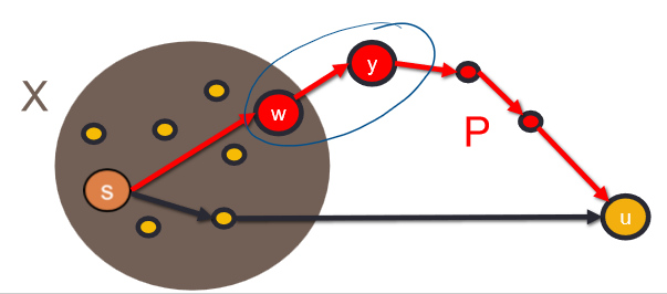
• $dist(w)=d(w)$ by the inductive hypothesis
• $dist(y)\ge dist(u)$ by choice of $u$ (Dijkstra always picks the minimum-dist vertex in $F$ next)

Therefore:

\begin{align*} d(u) &= \underbrace{ len(P) }_{ s \to u } \geq \underbrace{ dist(w) + \ell(w,y) }_{ s \to y } \ &= dist(y) \geq dist(u) > d(u)\ &\therefore \boxed{d(u) > d(u)} \end{align*}

This is a contradiction, so the negation of our assumption must be true: $dist(u)=d(u)$. $■$

---

Time & Space Complexity Analysis

General Case

Total runtime is:

$O(|V|(\text{deletemin})+|E|(\text{decreasekey}))$

Different implementations of Priority Queue have different trade-offs between the costs of deletemin and decreasekey. There isn't a single implementation that's optimal for all kinds of graphs.

Implementation-Dependent Variations

Array as a Priority Queue

Indexed by vertices, giving key value directly (e.g. Array[A] = 2, Array[B] = 9, …).

• deletemin: $O(|V|)$ — need to scan through the array to find which node contains the smallest distance
• decreasekey: $O(1)$ — array access by index means you can immediately find and update the (key, value) pair

Total Runtime:

$|V|\times deletemin+|E|\times decreasekey=|V|\times O(|V|)+|E|\times O(1)=\boxed{O(|V{|}^2)}$

Binary Heap as Priority Queue

Binary Heap A complete binary tree of objects (vertices) with the property that each key value of an object is less than or equal to the key value of its children.

• Can be implemented with an array $a[n]$ of vertices
• The children of $a_i$ are $a_{2i}$ and $a_{2i+1}$
• The parent of $a_i$ is $a_{\lfloor i/2\rfloor }$

• deletemin: The minimum key is guaranteed to be the root. Removing it requires replacing the root with the last object and letting it trickle down — $O(\log n)$ where $n=|V|$, so $O(\log |V|)$.
• decreasekey: Decreasing a key may require the object to bubble up — $O(\log n)$ where $n=|V|$, so $O(\log |V|)$.

How do we know where $v$ is in the binary heap? Keep a supplemental array (address book) indexed by $v$, with pointers in both directions between this array and the binary heap elements.

Total Runtime:

$|V|\times deletemin+|E|\times decreasekey=|V|\times O(\log |V|)+|E|\times O(\log |V|)=\boxed{O((|V|+|E|)\log |V|)}$

Priority Queue Operations Overview

	What it does	Array Implementation	Heap Implementation	Number of Operations
insert	Add a new element with its priority value to the queue	$O(1)$ — just append to end	$O(\log n)$ — add to end, then bubble up	$n$
deletemin	Extract the unvisited vertex with the smallest distance	$O(n)$ — must scan entire array to find minimum	$O(\log n)$ — remove root, move last to the top, bubble down	$n$
decreasekey	If you find a shorter path to a vertex, update its distance in the queue	$O(1)$ — access by index	$O(\log n)$ — update value, bubble up	$\Vert E\Vert$

When to Use Which Implementation

	Array $O(\Vert V{\Vert }^2)$	Binary Heap $O((\Vert V\Vert +\Vert E\Vert )\log \Vert V\Vert )$
Sparse Graphs: $\Vert E\Vert =\Theta (\Vert V\Vert )$	✘	✔
Dense Graphs: $\Vert E\Vert =\Theta (\Vert V{\Vert }^2)$	✔	✘

Best / Worst / Average Case

• Best / Worst / Average case: All the same order for a given PQ implementation — Dijkstra always processes every vertex once (deletemin) and considers every edge once (decreasekey/relaxation attempt), so there’s no early-exit case that changes the asymptotic bound.

---

Drawbacks / Constraints

• Preconditions: Requires all edge weights to be non-negative.
• The Negative Weight Problem: Dijkstra’s Algorithm does not work with negative edge weights.
  • The Reason: Dijkstra assumes that once a node is marked “Done,” no future path can possibly be shorter.
  • The Failure: A negative edge could “reduce” the cost of a path discovered later, breaking the greedy assumption.
• Not suitable for: Graphs with negative edge weights — use Bellman-Ford Algorithm instead.
• Alternatives to consider: Breadth First Search (BFS) if all edges have equal weight (simpler, same $O(V+E)$ runtime without needing a priority queue).

---

Comparison of Shortest Path Algorithms

Algorithm	Graph Type	Guaranteed Shortest Path?
BFS	Unweighted	Yes (by edge count)
DFS	Any	No
Dijkstra	Weighted (Positive only)	Yes (by total weight)

---

References / Links

• Breadth First Search (BFS)
• Depth First Search (DFS)
• Bellman-Ford Algorithm
• Priority Queue