Binary Search Tree (BSTs)

ABSTRACT

While a Heap provides $O(1)$ access to the highest-priority element, it is inefficient for finding arbitrary values. A Binary Search Tree solves this by maintaining a sorted structure that allows for fast searching, similar to Binary Search in an Array.

1. Core Properties

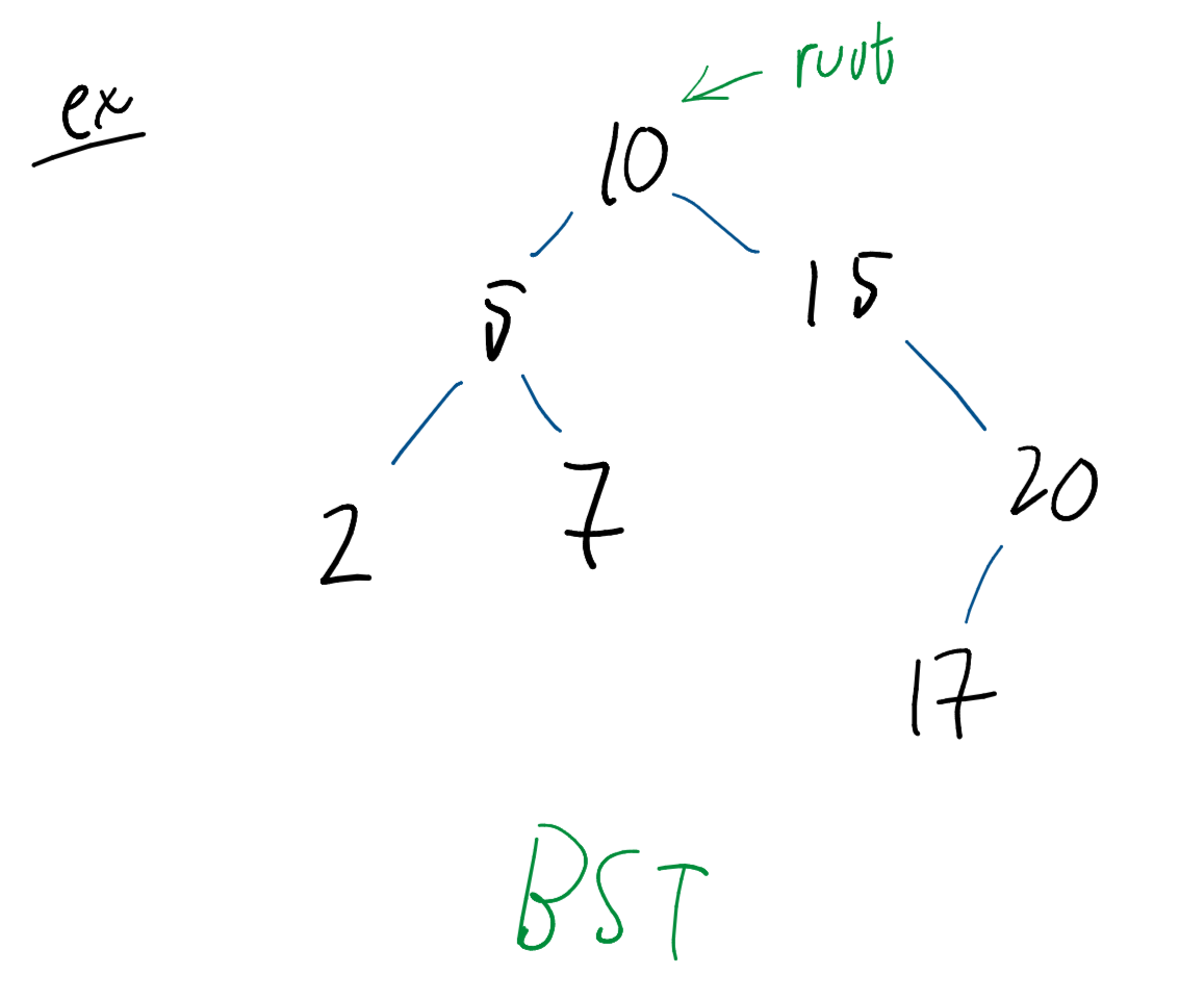
A BST is a rooted binary tree that must satisfy the BST Property:

• For any given node, all nodes in its left subtree have smaller values.
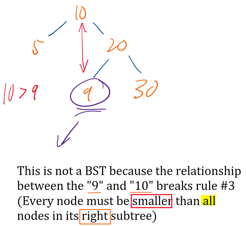
• All nodes in its right subtree have larger values.
• This implies that the tree cannot contain duplicate elements.

---

2. Basic Operations

BST operations are typically proportional to the height ($h$) of the tree.

find(element)

Used to check if a specific value exists within the tree. It leverages the BST property to achieve $O(h)$ time complexity.

find(element): // returns True if element exists in BST, otherwise returns False
    current = root                 // start at the root
    while current != element:
        if element < current:      // if element < current, traverse left
            current = current.leftChild
        else if element > current: // if element > current, traverse right
            current = current.rightChild
        if current == NULL:        // if we traversed and there was no such child, failure
            return False
    return True // we only reach here if current == element, which means we found element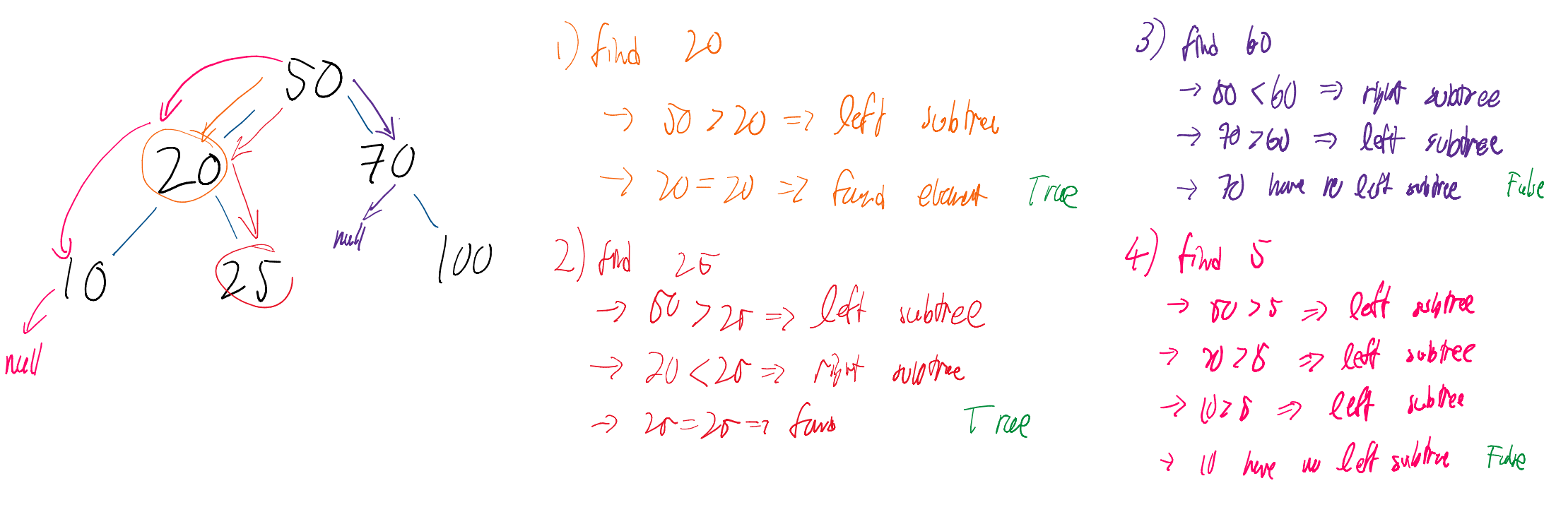

insert(element)

Adds a new node to the tree. It traverses the tree until it finds a NULL child where the element should logically reside.

insert(element): // inserts element into BST and returns True on success (or False on failure)
    if no elements exist in the BST:       // empty tree, so element becomes the root
        root = element
        size = size + 1
        return True
    current = root                         // start at the root
    while current != element:
        if element < current:
            if current.leftChild == NULL:  // if no left child exists, insert element as left child
                current.leftChild = element
                size = size + 1
                return True
            else:                          // if a left child does exist, traverse left
                current = current.leftChild
        else if element > current:
            if current.rightChild == NULL: // if no right child exists, insert element as right child
                current.rightChild = element
                size = size + 1
                return True
            else:                          // if a right child does exist, traverse right
                current = current.rightChild
    return False // we only reach here if current == element, and we can't have duplicate elements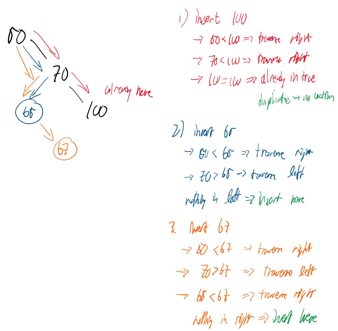

clear()

Resets the tree by removing the reference to the root and resetting the counter.

clear(): // clears BST
    root = NULL
    size = 0

size()

Returns the total number of nodes currently stored in the BST.

size(): // returns the number of elements in BST
    return size

empty()

A boolean check to see if the tree contains any data.

empty(): // returns True if BST is empty, otherwise returns False
    if size == 0:
        return True
    else:
        return False

---

3. Successor and Removal Logic

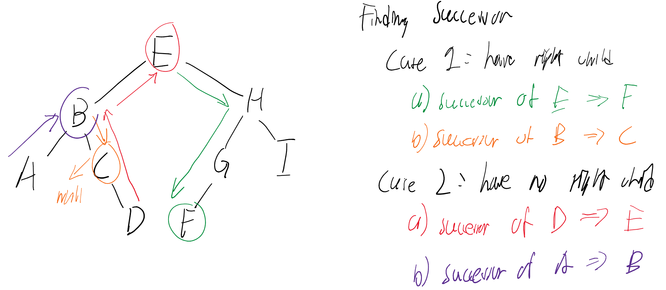
Finding the Successor

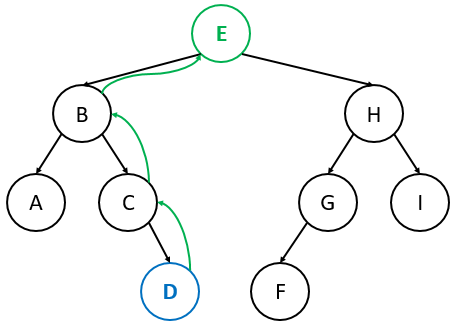
The successor of a node $u$ is the next largest node in the BST.

• Case 1 (Right child exists): The successor is the left-most node of $u$‘s right subtree.

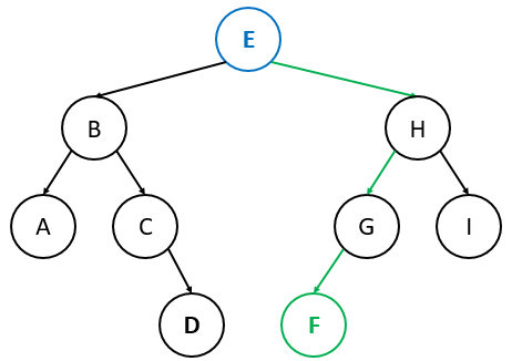
• Case 2 (No right child): Traverse up until you find a node that is the left child of its parent. That parent is the successor.

successor(u): // returns u's successor, or NULL if u does not have a successor
    if u.rightChild != NULL:             // Case 1: u has a right child
        current = u.rightChild
        while current.leftChild != NULL: // find the smallest node in u's right subtree
            current = current.leftChild
        return current
    else:                                // Case 2: u does not have a right child
        current = u
        while current.parent != NULL:    // traverse up until current node is its parent's left child
            if current == current.parent.leftChild:
                return current.parent
            else:
                current = current.parent
        return NULL // we have reached the root and didn't find a successor, so no successor exists

Examples

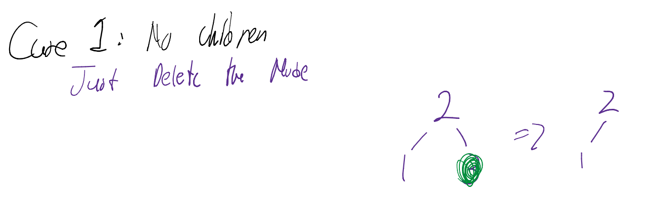
Removal Cases

1. Zero Children (Leaf): Simply delete the node.

2. One Child: Connect the node’s parent directly to its child.

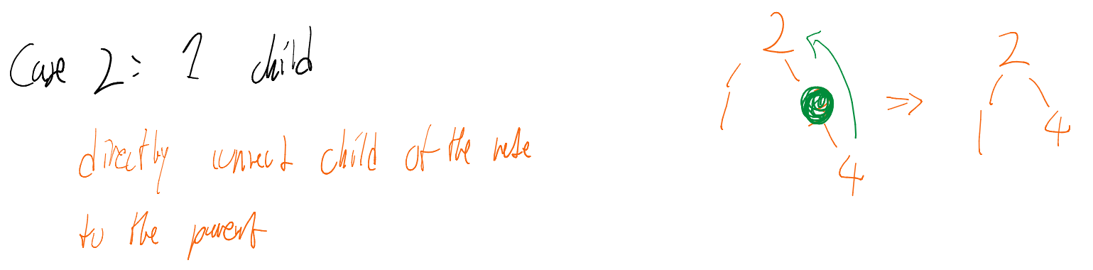
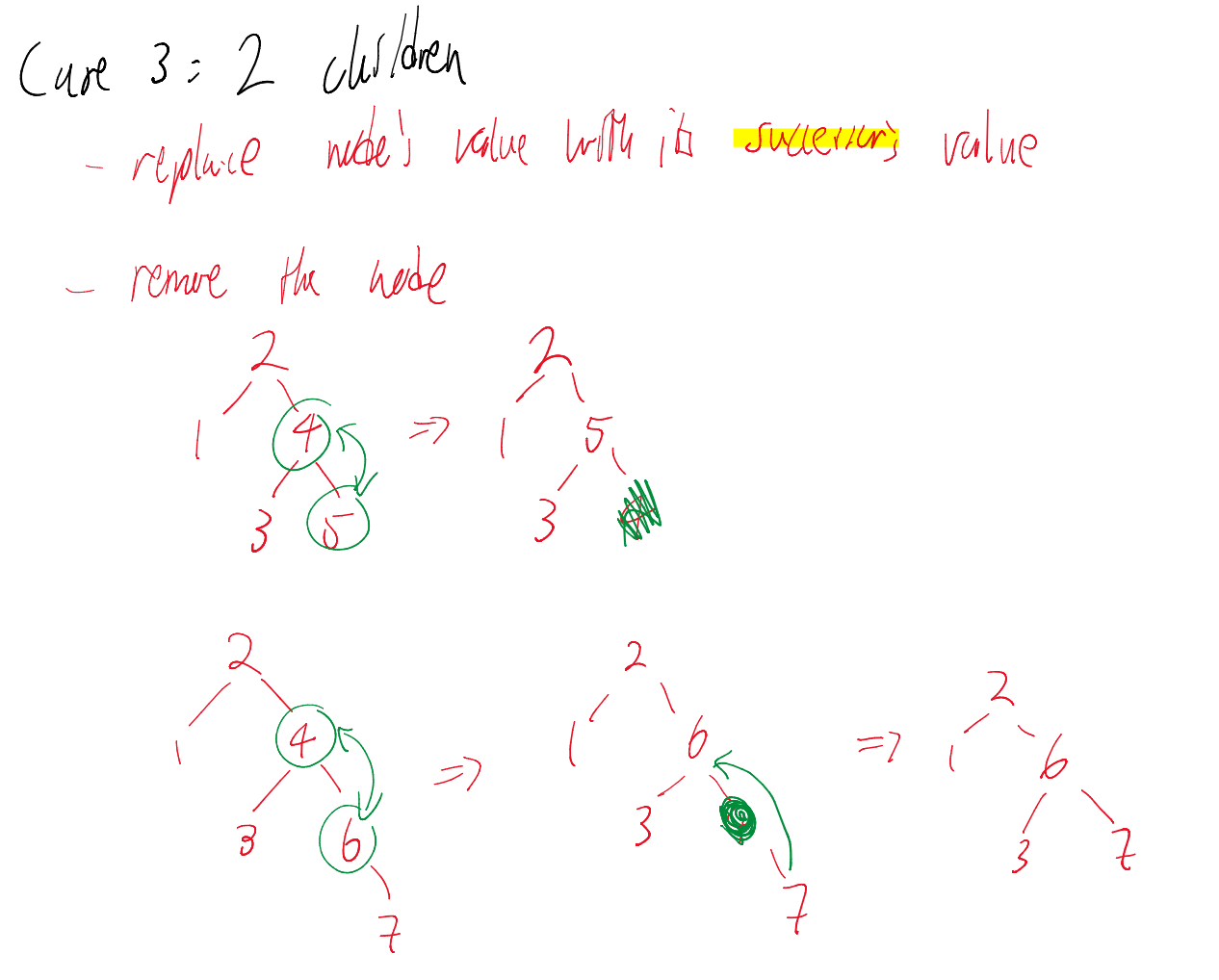
3. Two Children: Find the node’s successor, replace the node’s value with the successor’s value, and then delete the successor (which is guaranteed to have at most one child).

remove(element): // removes element if it exists in BST (returns True), or returns False otherwise
    current = root                 // start at the root
    while current != element:
        if element < current:      // if element < current, traverse left
            current = current.leftChild
        else if element > current: // if element > current, traverse right
            current = current.rightChild
        if current == NULL:        // if we traversed and there was no such child, failure
            return False
    // we only reach here if current == element, which means we found element
    if current.leftChild == NULL and current.rightChild == NULL:     // Case 1 (no children)
        remove the edge from current.parent to current
    else if current.leftChild == NULL or current.rightChild == NULL: // Case 2 (one child)
        have current.parent point to current’s child instead of to current
    else:                                                            // Case 3 (two children)
        s = current’s successor
        if s is its parent's left child:
            s.parent.leftChild = s.rightChild  // s.rightChild will either be NULL or a node
        else:
            s.parent.rightChild = s.rightChild // s.rightChild will either be NULL or a node
        replace current's value with s's value

---

4. Traversals

An In-Order Traversal visits nodes in the sequence: Left $\to$ Current $\to$ Right.

• Result: This always visits nodes in sorted order.
• Algorithm: Start at the left-most element and repeatedly call the successor() function.

inOrder(): // perform an in-order traversal over the elements of BST using successor()
    current = the left-most element of BST
    while current != NULL:
        output current
        current = successor(current)

---

5. Performance and Balance

The efficiency of a BST is entirely dependent on its Shape, which is determined by the order in which elements are inserted.

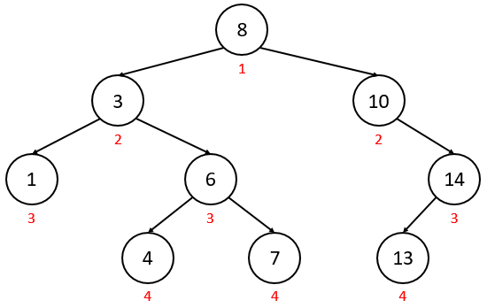
Tree Height ($h$)

The number of edges from the root to the deepest leaf.

• Empty Tree: $h=-1$
• Single Node: $h=0$
• Worst Case: $h=n-1$ (where $n$ is the number of nodes).

Detailed Balance Comparison

Feature	Perfectly Balanced	Self-Balancing (AVL/RB)	Degenerate (Unbalanced)
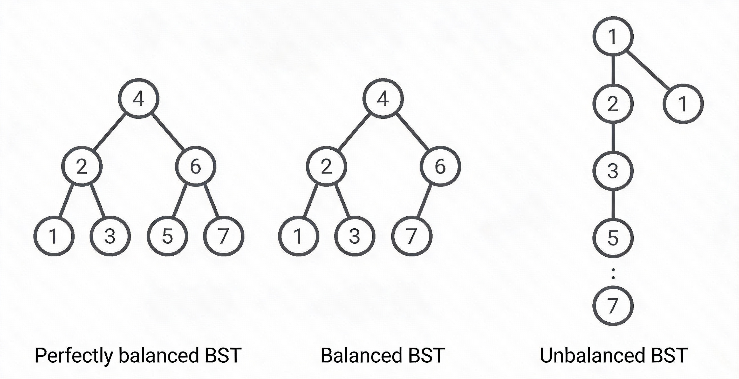
Visual Shape	Full, symmetrical triangle.	Mostly full; slight height differences allowed.	A straight line (resembles a Linked List).
Logic	Every level is filled before starting a new one.	Stricter rules ($BF\le 1$) keep height near-optimal.	Nodes are added only to one side.
Height	$\approx {\log }_2(n)$	$O(\log n)$	$O(n)$
Search Time	$O(\log n)$ (Fastest)	$O(\log n)$ (Guaranteed)	$O(n)$ (Slowest)
In-Practice	Rare/Hard to maintain.	The Industry Standard.	Happens with sorted data.

The Three “States” of a BST

1. The Ideal: Perfectly Balanced

A tree where all leaves are at the same depth or differ by at most one level, and every internal node has exactly two children. While this provides the absolute minimum $h$, it is computationally expensive to keep a tree “perfect” after every insertion or deletion.

2. The Standard: Height-Balanced

This is what we usually mean when we say a “Balanced Tree.” Data structures like AVL Trees or Red-Black Trees don’t have to be perfect; they just need to ensure the height remains logarithmic.

• AVL Rule: The heights of the left and right subtrees of any node differ by at most 1.
• Performance: You get $O(\log n)$ speed without the massive overhead of keeping the tree “perfect.”

3. The Failure: Degenerate (Skewed)

This happens when the BST property is technically satisfied, but the structure fails. If the tree only grows in one direction, you lose the “branching” power of the tree.

The Insertion Order Trap

If you insert elements into a standard BST in sorted order (e.g., 1, 2, 3, 4, 5) or reverse sorted order, the tree will become perfectly unbalanced.

• Result: Your “Search Tree” is now a Linked List.

• Fix: This is why we use AVL or Red-Black Trees, which use “rotations” to force the tree back into a balanced shape regardless of insertion order.

---

6. Average-Case Performance Analysis

While the worst-case height of a BST is $O(n)$, the average case is significantly more efficient. Under specific conditions, the expected time complexity for a successful find operation is $O(\log n)$.

6.1 The Assumptions

To formally prove the average-case complexity, we make two key assumptions:

1. Uniform Search Probability: All $n$ elements in the tree are equally likely to be the target of a search.
2. Uniform Insertion Probability: All $n!$ possible insertion orders (permutations) of the elements are equally likely.

6.2 Defining Expected Depth

We define the depth of node $i$ ($d_i$) as the number of nodes along the path from the root to node $i$.

• The root has a depth of $1$.
• “Average-case time complexity” is equivalent to computing the expected depth of a node in a BST with $n$ nodes.

Recall

From statistics, the expected value of a discrete random variable $X$ is

$$\sum _{i=1}^n{p}_i{X}_i$$

where $p_i$ is the probability that outcome $X_i$ occurs

For more information, visit Expected Value

For a specific BST $j$, the expected depth $E_j(d)$ is:

$$E_j(d)=\frac{1}{n}\sum _{i=1}^n{d}_{ji}=\frac{1}{n}{D}_j(n)$$

where $D_j(n)$ = Total Depth of tree $j$.

To find the average across all trees, we solve for $D(n)$, the expected total depth among all possible BSTs.

6.3 Calculating Expected Total Depth

Let $D(n)$ denote the expected total depth among ALL BSTs with $n$ nodes.

We can find each BST $j$ as the result of insertion order $j$ since a BST can be defined by the order in which we inserted its elements

• First Insertion: insert any of our first $n$ elements
• Second Insertion: insert any of the $n-1$ remaining elements

If we continue this pattern, there are $n\cdot (n-1)\cdot (n-2)\cdot \cdots =n!$ possible insertion orders.

According to our second assumption, all insertion orders are equally likely. Therefore we could rewrite $D(n)$ to be:

$$D(n)=\frac{1}{n!}\sum _{j=1}^{n!}{D}_j(n)$$

This approach is far too inefficient

6.4 The Recurrence Relation

Instead of brute-forcing all $n!$ trees, we use a recurrence relation based on the root’s position. If the root is the $(i+1{)}^{th}$ smallest element, there are $i$ nodes in the left subtree and $n-i-1$ nodes in the right subtree.

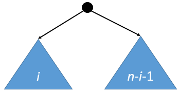
The expected total depth given $i$ nodes in the left subtree is:

$$D(n|i)=D(i)+D(n-i-1)+n$$

(The $+n$ accounts for the fact that every node in the subtrees is now one level deeper due to the new root ancestor).

Note

$i$ can be

• at minimum $0$ → there is a possibility that there is no left/right subtree
• at maximum $n-1$ → there is a possibility that all nodes (aside from the root) is in left/right subtree

Since every element is equally likely to be the first one inserted (the root), the probability of any specific $i$ is $1/n$. This gives us:

$$D(n)=\frac{2}{n}\sum _{i=0}^{n-1}D(i)+n$$

6.5 Mathematical Solution

By manipulating the recurrence (multiplying by $n$, substituting $n-1$, and subtracting the equations), we arrive at a telescoping form:

$$nD(n)=(n+1)D(n-1)+2n-1$$

Solving this results in the closed-form solution:

$$D(n)=2(n+1)\sum _{i=1}^n\frac{1}{i}-3n$$

Final Approximation

Using the harmonic series approximation (${\sum }_{i=1}^n\frac{1}{i}\approx \ln n$), the average-case number of comparisons for a successful find is:

$$\frac{D(n)}{n}\approx 2\ln n\approx 1.386{\log }_{2}n$$

Since $1.386$ is a constant, we have formally proven that the average-case complexity is $O(\log n)$.

6.6 Limitations and Self-Balancing Trees

In practice, real-life data often violates the assumption of random insertion order. For example, inserting pre-sorted data leads to a “degenerate” tree (essentially a Linked List).

To guarantee $O(\log n)$ performance regardless of insertion order, we use Self-Balancing Trees:

• Randomized Search Trees (Treap, RST): Uses random priorities to simulate random insertion order.
• AVL Tree: Uses height-based rotations to maintain balance.
• Red-Black Tree: Uses color-coding rules to ensure the tree remains roughly balanced.