Asymptotic Notation

ABSTRACT

Asymptotic notation provides a mathematical framework for describing the limiting behavior of functions. In computer science, we use it to classify the efficiency of algorithms by comparing their growth rates to standard functions (like $n^2$ or $\log n$).

---

1. The Necessity of Efficiency: Turing’s Lesson

The history of computer science highlights that a correct algorithm is not always a “good” one. During WWII, Alan Turing’s team needed to crack the German Enigma code.

• The Problem: The Enigma machine changed its cipher every 24 hours. A machine that found the key in 48 hours was effectively useless.
• The Breakthrough: By using “pruning” logic (omitting solutions based on known phrases), Turing reduced the time complexity of the decryption, allowing the machine to finish within the required window.
• The Lesson: Algorithms must be quantified by how they scale as input size ($n$) grows.

---

2. Core Asymptotic Notations

To discuss efficiency scientifically, we use specific notations to define upper, lower, and tight bounds.

Notation	Intuition	Limit Definition limn→∞​g(n)f(n)​
Big-Theta ($\Theta$)	Same growth rate	$c$ (where $0<c<\infty$)
Big-O ($O$)	Same or better (Upper bound)	$c$ (where $0\le c<\infty$)
Big-Omega ($\Omega$)	Same or worse (Lower bound)	$c>0$ or $\infty$
Small-o ($o$)	Strictly better (Strict upper bound)	$0$

---

3. Mathematical Definitions

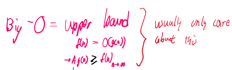
Big-O ($O$): The Upper Bound

$f(n)\in O(g(n))$ means $f(n)$ grows no faster than $g(n)$. This is the most common notation used in industry to describe worst-case scenarios.

• Formal Definition: There exist positive constants $C$ and $k$ such that $f(n)\le C\cdot g(n)$ for all $n\ge k$.
• Key Property: $f(n)+g(n)\in O(\max \{f(n),g(n)\})$.

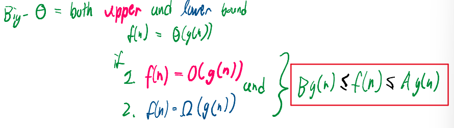
Big-Theta ($\Theta$): The Tight Bound

$f(n)\in \Theta (g(n))$ means $f(n)$ and $g(n)$ scale at the same rate.

• Formal Definition: There exist positive constants $C,C^{\prime }$, and $k$ such that $C^{\prime }g(n)\le f(n)\le Cg(n)$ for all $n\ge k$.

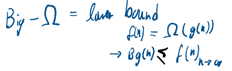
Big-Omega ($\Omega$): The Lower Bound

$f(n)\in \Omega (g(n))$ means $f(n)$ grows at least as fast as $g(n)$.

• Limit Test: If ${\lim }_{n\to \infty }\frac{f(n)}{g(n)}=c>0$ or $\infty$, then $f(n)\in \Omega (g(n))$.

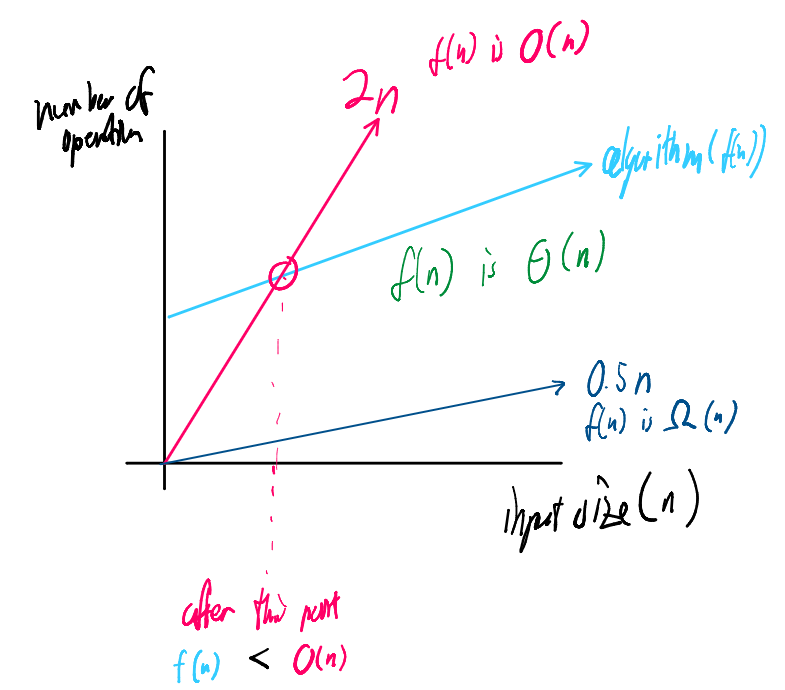
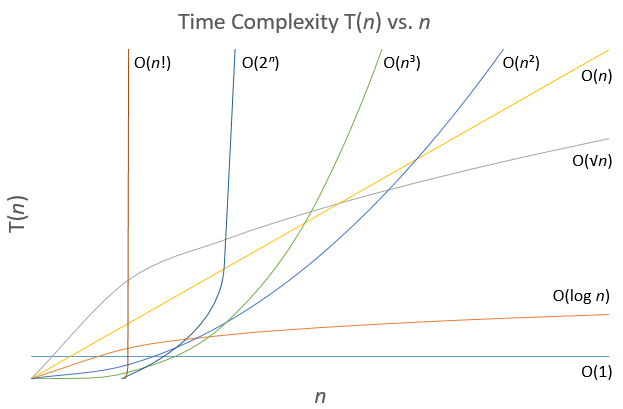
Graph Comparison

---

4. Hierarchy of Growth Rates

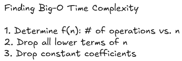
When analyzing algorithms, we simplify functions by dropping constants and lower-order terms. The following standard functions are ordered from slowest to fastest growth:

$1\ll \log n\ll n\ll n\log n\ll n^2\ll n^3\ll 2^n\ll n!$

Term	Complexity	Verdict
Constant	$O(1)$	Excellent
Logarithmic	$O(\log n)$	Excellent
Linear	$O(n)$	Good
Polynomial	$O(n^k)$	Fair
Exponential	$O(k^n)$	Poor
Factorial	$O(n!)$	Unusable for large $n$

---

5. Time vs. Space Complexity

• Time Complexity: Quantifies execution time by counting elementary operations.
• Space Complexity: Measures the amount of working storage (memory) required for an input of size $n$.
  • Example: A matrix storing travel data between $n$ cities requires $2n^2$ storage, simplified to $O(n^2)$ space.

---

6. Practical Application

Example: Polynomial Bound

Prove $(3n^2+2n)\in O(n^2)$.

1. Choose $C=5$ and $k=1$.
2. For $n\ge 1$, we know $2n\le 2n^2$.
3. Thus, $3n^2+2n\le 3n^2+2n^2=5n^2$.
4. Since $f(n)\le 5g(n)$ for all $n\ge 1$, the claim is proven.