Circular Arrays

Definition

A Circular Array is a regular Array Lists with a clever implementation that mimics the properties of a Linked List. It treats the underlying linear array as a continuous ring by using head and tail indices.

• Head/Tail Indices: Instead of starting at index 0, the first element is at the head index and the last is at the tail index.
• Contiguity: Elements are contiguous in the logical sequence, even if they “wrap around” the physical end of the backing array.

Wrapping Logic

• Add to End: Increment tail. If it hits the end of the array, it wraps back to index 0.
• Add to Front: Decrement head. If it hits -1, it wraps to the last index (size - 1).

---

System Representations

There are two primary ways to conceptualize a Circular Array. Both are equally valid and describe the same underlying logic.

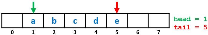
1. The Physical (Linear) View

This representation shows how the data actually sits in computer memory. The head and tail indices move across the array and “wrap” back to the other side when they hit the boundaries.

• Wrap to Front: If tail reaches the end (size), it wraps to index 0.
• Wrap to Back: If head drops below 0, it wraps to index size−1.

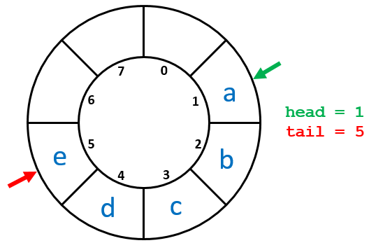
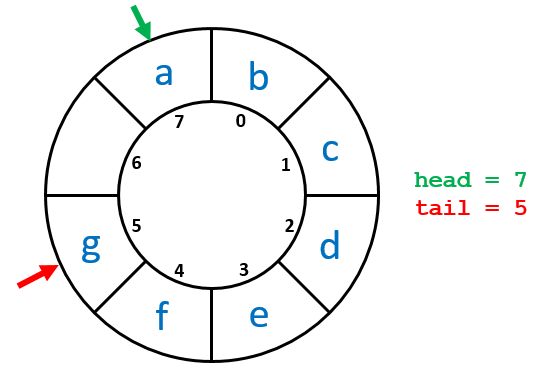
2. The Logical (Circular) View

Since we only care about an element’s location relative to the head and tail, many prefer to visualize the structure as a ring. In this view, the “wrap around” is a natural part of the circular path.

---

Insertion and Resizing

When the backing array becomes full, it must be resized. Similar to a standard Array List, we double the size and copy the elements.

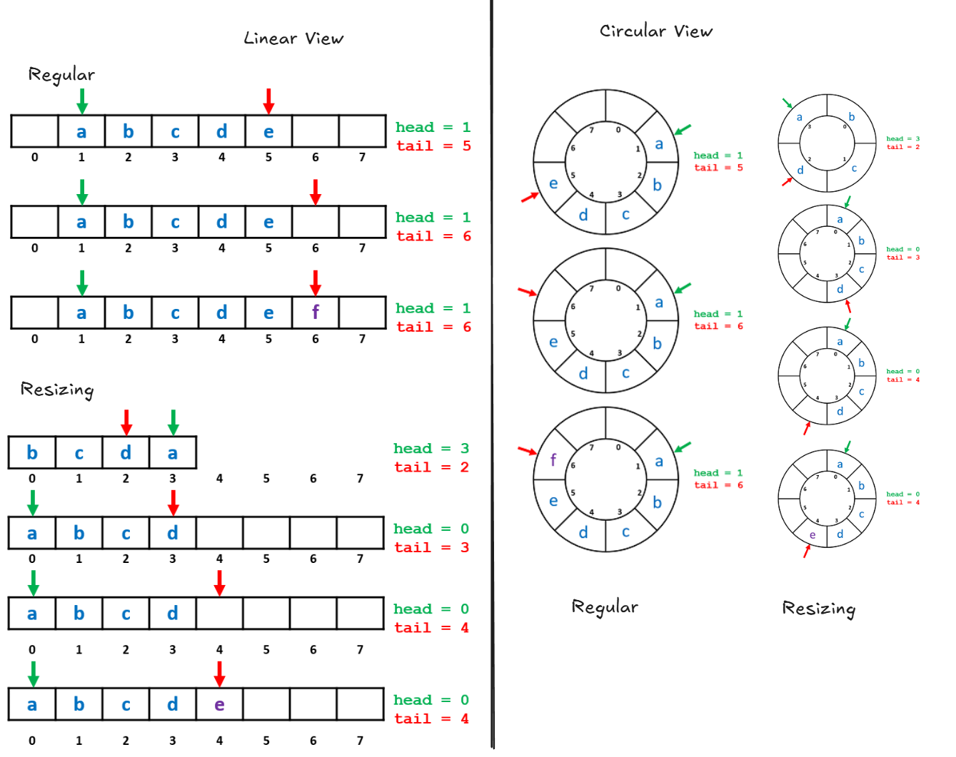
During a resize, you must "unroll" the circular structure so the new array begins with the head element at index 0.

# Check and resize if full
checkSize():
    if n == array.length:
        newArray = empty array of length 2*array.length
        for i from 0 to n-1:
            # Copy using modular mapping
            newArray[i] = array[(head + i) % array.length]
        array = newArray
        head = 0
        tail = n - 1
 
# Insert at the front
insertFront(element):
    checkSize()
    head = head - 1
    if head == -1:
        head = array.length - 1
    array[head] = element
    n = n + 1
 
# Insert at the back
insertBack(element):
    checkSize()
    tail = tail + 1
    if tail == array.length:
        tail = 0
    array[tail] = element
    n = n + 1

---

Removal

• Remove Front: Erase the element at head and increment the head index (wrapping if necessary).
• Remove Back: Erase the element at tail and decrement the tail index (wrapping if necessary).

def removeFront():
    # erase array[head] (optional for non-pointers)
    head = (head + 1) % array.length
    n = n - 1
 
def removeBack():
    # erase array[tail]
    tail = tail - 1
    if tail == -1:
        tail = array.length - 1
    n = n - 1

Is it necessary to perform the "erase" steps?

Answer pointers, you must explicitly deallocate or null them to prevent memory leaks.

Usually no; the values will simply be overwritten by new insertions. However, if the array stores

---

Finding and Random Access

Unlike a Linked List, a Circular Array maintains Random Access. To access logical element i, you calculate the physical index:

$$(head+i)\mathrm{mod}array.length$$

When can we omit the modulo operation?

Answer $(head+i)<array.length$.

When

---

Performance Summary

Operation	Complexity	Note
Random Access	O(1)	Achieved via modular arithmetic.
Insert/Remove Front	O(1)	No shifting required (unlike Array Lists).
Insert/Remove Back	O(1)	Direct index adjustment.
Resize	O(n)	Occurs infrequently (amortized O(1)).

Conclusion: Circular Arrays provide the efficient end-manipulation of a Linked List while retaining the O(1) random access of an Array List. This makes them ideal for implementing structures like Double-Ended Queues (Deques).