Closed Addressing (Separate Chaining)

ABSTRACT

Separate Chaining (also known as Closed Addressing) is a collision resolution strategy where each slot in the hash table points to a separate data structure—most commonly a Linked List. Unlike Open Addressing (Linear Probing), where collisions force keys into different slots, Separate Chaining keeps keys at their original hashed index.

---

1. The Core Concept: Open Hashing

In Linear Probing, a collision fills an empty slot elsewhere in the array, which directly increases the probability of future collisions.

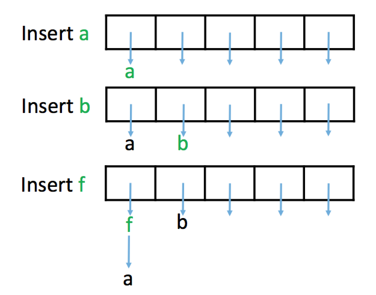
In Separate Chaining, the array doesn’t store the keys themselves. Instead, it stores “buckets” (pointers to Linked Lists). When a collision occurs, the new key is simply appended to the list at that specific index.

Why “Closed Addressing”?

• Closed Addressing: The key is “closed” to its original hashed address; it never moves to a different index.
• Open Hashing: The hashing is “open” because the data is stored outside the primary array structure.

---

2. Implementation & Logic

Insertion Algorithm

When inserting a key $k$:

1. Calculate the index: index = H(k).
2. Check for duplicates in the list at arr[index].
3. If no duplicate exists, insert $k$ into the list.
4. Resizing: If the Load Factor ($\alpha =N/M$) exceeds a threshold (typically 0.75 to 1.0), create a larger prime-sized array and re-hash all elements.

insert_SeparateChaining(k): // Insert k using Separate Chaining for collision resolution
 
    index = H(k)
 
    // check for duplicate insertions (not allowed) and perform insertion
    if Linked List in arr[index] does not contain k:
        insert k into Linked List at arr[index]; n = n+1
 
        // resize backing array (if necessary)
        if n/m > loadFactorThreshold:
           arr2 = new array with a size ~2 times the size of arr that is prime  // new backing array
           insert all elements from arr into arr2 using normal insert algorithm // rehash all elements
           arr = arr2; m = length of arr2                                       // replace arr with arr2
 
        return true  // successful insertion
 
    else:
        return false // unsuccessful insertion

The core of the Separate Chaining algorithm is defined by this line:

insert k into Linked List at arr[index]

Handling Duplicates

There are two primary ways to manage duplicate keys:

• Insert-time check: Scan the list during insert(). If the key exists, do nothing. (Slows down insertion, speeds up deletion). $✓$
• Delete-time check: Always insert at the head. Scan the entire list during remove() to ensure all copies are deleted. (Speeds up insertion, slows down deletion).

---

3. Beyond Linked Lists

While Linked Lists are the most common choice, buckets can also be implemented using:

• AVL Trees / Red-Black Trees: Reduces the worst-case search time from $O(N)$ to $O(\log N)$ for a single bucket.
• Dynamic Arrays: Better cache locality than linked lists but more expensive to resize.

TIP

If a single bucket becomes so long that it requires a Balanced BST to remain fast, it usually indicates a poor hash function or a low capacity, which should be addressed first.

---

4. Pros and Cons

Advantages

• Simple Deletion: Unlike Open Addressing (Linear Probing), which requires “Lazy Deletion” (tombstones), you can simply remove a node from the linked list.
• Graceful Degradation: The table never actually “fills up.” Performance slows down as lists grow longer, but insertions always succeed.
• Collision Probability: A collision at index $i$ does not increase the chance of a collision at index $i+1$.

Disadvantages

• Memory Overhead: Storing pointers for every node requires extra memory.
• Cache Locality: Linked list nodes are scattered in memory. This causes Cache Misses, making the table slower than array-based methods in high-performance systems.

---

5. Summary of Collision Strategies

Feature	Open Addressing	Separate Chaining
Storage Location	Inside the array (Internal)	Outside the array (External Lists)
Max Load Factor ($\alpha$)	Must be $<1.0$ (Strictly limited)	Can be $>1.0$ (Table never “fills”)
Deletion	Complex (Requires “Tombstones”)	Simple (Standard List removal)
Clumping	High (Primary/Secondary Clustering)	Low (No inter-slot interference)
Memory Overhead	Low (Array only)	High (Pointers/Nodes for Lists)
Cache Performance	Excellent (High locality)	Poor (Nodes scattered in memory)