ABSTRACT
In complex social networks or connectivity problems—like CIA agent Sarah Walker tracking connections between Chuck Bartowski and known villains—standard graph traversals (BFS/DFS) can be too slow for frequent queries. The Disjoint Set ADT provides a way to merge groups and check connectivity in near-constant time.
1. The Core Operations: Union and Find
A Disjoint Set manages a collection of elements partitioned into non-overlapping (disjoint) subsets. It supports two primary operations:
- Find(): Determine which set belongs to. If , then and are connected.
- Union(): Merge the set containing with the set containing into a single set.
2. Implementation: The Up-Tree
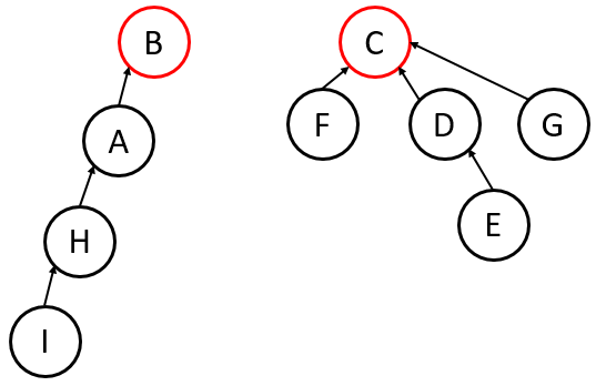
The most efficient way to represent these sets is using an Up-Tree. Unlike a standard tree where parents point to children, in an Up-Tree, children point to their parents.
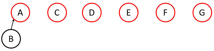
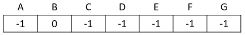
- Sentinel Nodes (Roots): The “representative” or “name” of the set. A node with no parent (or a self-pointer) is the root.
- Array Representation: We can store the entire forest in a single array.
Array[i]stores the index of the parent of .- If
Array[i] == -1(or a negative number), node is a sentinel node.
Example
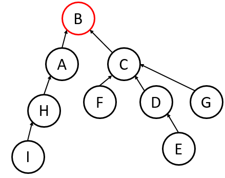
3. Optimizing the Union Operation
To keep the trees from becoming too tall (which makes Find slow), we use “smart” union strategies:
Union-by-Size
Always attach the root of the smaller tree (fewer nodes) to the root of the larger tree.
- Worst-case Height: .
- Benefit: Easy to track; just store the negative size in the sentinel’s array slot (e.g.,
-5means it’s a root of a set with 5 nodes).
Union-by-Height (Rank)
Always attach the shorter tree to the taller tree.
- Worst-case Height: .
- Drawback: Harder to maintain if you also use Path Compression (see below), as heights change during searches.
If we used Union-by-Size instead of Union-by-Height on the example above, would the resulting tree be better, worse, or just as good as the one produced by the Union-by-Height method?
In the provided example, Union-by-Size would likely produce a tree with the same or better performance than Union-by-Height, but in practice, Size is preferred because it is easier to update when we start moving nodes around during “Path Compression.”
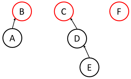
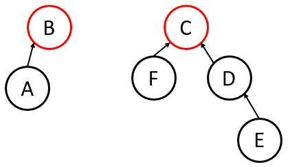
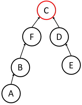
4. Optimizing the Find Operation: Path Compression
Every time you perform a Find(u), you traverse from up to the root.
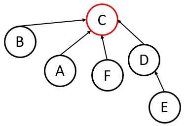
Path Compression dictates that after finding the root, you go back and reattach (and every node on the path) directly to the root.
- Result: The next time you call
Findon any of those nodes, it takes time. - Self-Adjustment: This turns the Up-Tree into a self-adjusting structure.
Sees the nodes along the traversal up
5. Amortized Cost Analysis
A. The “Investment” Logic
In standard analysis, we say a Find operation is , where is the height of the tree. If you have a poorly shaped tree, one Find could take time.
In Amortized Analysis, we considers the time or space cost of doing a sequence of operations (as opposed to a single operation) because the total cost of the entire sequence of operations might be less with the extra initial work than without! Acknowledging that the initial operation is actually an investment. As the algorithm travels up to the root, it performs extra work to reassign every node it touches to point directly to the root.
- The Cost: This specific
Findis “expensive” because of the extra pointer reassignments. - The Reward: Every future
Findfor any of those nodes (and their descendants) is now .
B. The Three Methods of Analysis
To prove that the amortized cost is nearly constant, computer scientists use three formal frameworks:
- The Aggregate Method: We show that for a sequence of operations, the total time is small. The amortized cost is simply .
- The Accounting (Banker’s) Method: We “charge” each cheap operation a bit more than it actually costs. We save this extra “money” as a credit in a bank account. When an expensive
Findoccurs, it “withdraws” those credits to pay for the work of compressing the path. - The Potential (Physicist’s) Method: We define a “potential function” that represents the “messiness” or height of the tree. A deep, uncompressed tree has high potential energy. An expensive
Findoperation performs work that significantly decreases the potential energy (by flattening the tree), which offsets the high actual cost of the operation.
C. The Scaling of
The reason the complexity is rather than just is because the tree isn’t perfectly flat immediately. However, (the iterative logarithm) is a function that grows so slowly it is essentially a constant for any data we can physically store.
| Total Elements (N) | log∗N |
|---|---|
| 2 | 1 |
| 4 () | 2 |
| 16 () | 3 |
| 65,536 () | 4 |
| (More than atoms in the universe) | 5 |
D. The “Nearly Constant” Result
The result of this analysis for Disjoint Sets is that the average cost per operation is .
The Inverse Ackermann Function is the mathematical way of saying: “This is technically not constant, but it grows so slowly that for any data set humanity will ever create, it will never exceed 5.”
Key Takeaway: Without amortized analysis, we would look at the worst-case of a single
Findand wrongly conclude the structure is inefficient. Amortized analysis reveals that the more you use the structure, the faster it gets, leading to a total runtime that is effectively linear ( for operations).
| Operation | Naive Implementation | With Union-by-Size & Path Compression |
|---|---|---|
| Union | ||
| Find |
Summary: Worst-Case Complexity of Disjoint Sets
While a single “find” or “union” operation can technically hit a worst-case of (with smart unioning) or (without), we use Amortized Analysis to describe the true performance over a sequence of operations.
- Total Complexity: For operations on a set of elements, the total worst-case time is __.
- Per-Operation Complexity: The “average” worst-case cost for a single operation is *, which is the Inverse Ackermann Function .
- The Result: Because grows so slowly that it never exceeds 5 for any practical value of , the complexity is considered effectively (constant time).